library(ggplot2)

te_paper  <- "#f5f4ee"
te_ink    <- "#16241d"
te_body   <- "#2c3a31"
te_forest <- "#275139"
te_rust   <- "#b5534e"
te_gold   <- "#c9b458"
te_line   <- "#dad9ca"

theme_datasheet <- function() {
  theme_minimal(base_size = 12) +
    theme(plot.background  = element_rect(fill = te_paper, colour = NA),
          panel.background = element_rect(fill = te_paper, colour = NA),
          panel.grid.major = element_line(colour = te_line, linewidth = 0.3),
          panel.grid.minor = element_blank(),
          text             = element_text(colour = te_body),
          plot.title       = element_text(colour = te_ink, face = "bold"),
          axis.text        = element_text(colour = te_body))
}

n_occ  <- 6
n_true <- 200
p_flat  <- 0.30
p_by_occ <- c(0.15, 0.45, 0.20, 0.40, 0.25, 0.35)
p_first <- 0.35
p_again <- 0.15

gen_m0 <- function(N, p) matrix(rbinom(N * n_occ, 1, p), N, n_occ)
gen_mt <- function(N, pv) sapply(pv, function(p) rbinom(N, 1, p))
gen_mb <- function(N, p, recap) {
  X <- matrix(0, N, n_occ); caught <- rep(FALSE, N)
  for (j in seq_len(n_occ)) {
    X[, j] <- rbinom(N, 1, ifelse(caught, recap, p))
    caught <- caught | X[, j] == 1
  }
  X
}
gen_mh <- function(N, a, b) {
  pi_ind <- rbeta(N, a, b)
  matrix(rbinom(N * n_occ, 1, rep(pi_ind, n_occ)), N, n_occ)
}Capture heterogeneity: Mt, Mb and Mh in R
R
capture-recapture
abundance
model diagnostics
ecology tutorial
Closed capture-recapture in R: the failures of constant capture probability cost different amounts. A trap response inflates abundance, heterogeneity cuts it.
Closed population capture-recapture starts from an assumption nobody believes: that every animal in the population has the same probability of being caught on every occasion. That is model M0, and it is the model whose arithmetic is short enough to write out. Otis and colleagues set out the family of alternatives in 1978, and the three that matter are named after the way the assumption fails. Mt lets the probability differ between occasions. Mb lets it change after an animal has been caught once. Mh lets it differ between individuals.
The site already has M0 and the standard closed population estimators. What it does not have is a measurement of what happens when M0 is fitted to data generated by each of the others, which is the situation every real study is in, because none of the three violations can be ruled out from the field.
The three do not cost the same, and two of them push in opposite directions. This post generates data under each, fits all four models by writing the likelihoods out, and measures both the bias and whether model selection can find the right one.
Four generators
Six occasions, two hundred animals, and a capture history matrix.
The four generators share a mean capture probability near 0.30 so that the number of animals ever seen is similar in all of them. What differs is where the variation sits.
Four likelihoods
Each model has the same structure: a combinatorial term for which animals were seen, the probability of every observed history, and the probability of the all zero history raised to the number never seen. The unknown abundance enters as the number of animals that produced the all zero history.
nll_m0 <- function(par, x, n_seen) {
  N <- n_seen + exp(par[1]); p <- plogis(par[2])
  -(lgamma(N + 1) - lgamma(N - n_seen + 1) +
      sum(x) * log(p) + (N * n_occ - sum(x)) * log(1 - p))
}
nll_mt <- function(par, X, n_seen) {
  N <- n_seen + exp(par[1]); pv <- plogis(par[-1]); cj <- colSums(X)
  -(lgamma(N + 1) - lgamma(N - n_seen + 1) +
      sum(cj * log(pv) + (n_seen - cj) * log(1 - pv)) +
      (N - n_seen) * sum(log(1 - pv)))
}
nll_mb <- function(par, X, n_seen) {
  N <- n_seen + exp(par[1]); p <- plogis(par[2]); recap <- plogis(par[3])
  first <- apply(X, 1, function(h) which(h == 1)[1])
  n_first  <- n_seen
  risk_p   <- sum(first) + (N - n_seen) * n_occ
  n_recap  <- sum(X) - n_seen
  risk_c   <- sum(n_occ - first)
  -(lgamma(N + 1) - lgamma(N - n_seen + 1) +
      n_first * log(p) + (risk_p - n_first) * log(1 - p) +
      n_recap * log(recap) + (risk_c - n_recap) * log(1 - recap))
}
nll_mh <- function(par, x, n_seen) {
  N <- n_seen + exp(par[1]); a <- exp(par[2]); b <- exp(par[3])
  hist_p <- function(k) lbeta(a + k, b + n_occ - k) - lbeta(a, b)
  -(lgamma(N + 1) - lgamma(N - n_seen + 1) +
      sum(hist_p(x)) + (N - n_seen) * hist_p(0))
}

fit_all <- function(X) {
  seen <- X[rowSums(X) > 0, , drop = FALSE]
  n_seen <- nrow(seen); x <- rowSums(seen)
  f0 <- optim(c(log(5), 0), nll_m0, x = x, n_seen = n_seen)
  ft <- optim(c(log(5), rep(0, n_occ)), nll_mt, X = seen, n_seen = n_seen,
              control = list(maxit = 2000))
  fb <- optim(c(log(5), 0, 0), nll_mb, X = seen, n_seen = n_seen,
              control = list(maxit = 2000))
  fh <- optim(c(log(5), 0, 0), nll_mh, x = x, n_seen = n_seen,
              control = list(maxit = 3000))
  singles <- sum(x == 1)
  c(M0 = n_seen + exp(f0$par[1]), Mt = n_seen + exp(ft$par[1]),
    Mb = n_seen + exp(fb$par[1]), Mh = n_seen + exp(fh$par[1]),
    jackknife = n_seen + singles * (n_occ - 1) / n_occ, seen = n_seen,
    aic_M0 = 2 * f0$value + 4, aic_Mt = 2 * ft$value + 2 * (1 + n_occ),
    aic_Mb = 2 * fb$value + 6, aic_Mh = 2 * fh$value + 6)
}
The jackknife on the last line is the classical estimator for individual heterogeneity from Burnham and Overton, and it is one line: add to the number of animals seen a correction driven by how many were caught exactly once.
What each violation costs
n_rep <- 60
scenarios <- list(
  "constant (M0)"          = function() gen_m0(n_true, p_flat),
  "time varying (Mt)"      = function() gen_mt(n_true, p_by_occ),
  "trap shy (Mb)"          = function() gen_mb(n_true, p_first, p_again),
  "heterogeneous (Mh)"     = function() gen_mh(n_true, 1.2, 2.8))

set.seed(3)
results <- lapply(scenarios, function(g) as.data.frame(t(replicate(n_rep, fit_all(g())))))

summary_row <- function(r) {
  aic <- as.matrix(r[, c("aic_M0", "aic_Mt", "aic_Mb", "aic_Mh")])
  picked <- c("M0", "Mt", "Mb", "Mh")[apply(aic, 1, which.min)]
  data.frame(M0 = median(r$M0), Mt = median(r$Mt), Mb = median(r$Mb),
             Mh = median(r$Mh), jackknife = median(r$jackknife),
             seen = median(r$seen),
             chosen = round(100 * mean(picked == "M0"), 0))
}
tbl <- do.call(rbind, lapply(results, summary_row))
tbl$truth_recovered <- round(100 * (tbl$M0 / n_true - 1), 1)
print(round(tbl[, c("seen", "M0", "Mt", "Mb", "Mh", "jackknife",
                    "truth_recovered")], 1))
seen M0 Mt Mb Mh jackknife truth_recovered
constant (M0) 177.0 201.5 201.4 200.1 203.4 228.9 0.8
time varying (Mt) 177.5 200.3 197.4 215.7 201.3 228.0 0.1
trap shy (Mb) 184.5 266.3 263.5 198.4 271.1 272.6 33.2
heterogeneous (Mh) 148.0 156.1 156.0 157.6 192.6 187.8 -22.0Read the M0 column against a true abundance of 200.
Time variation is nearly free. Capture probability swinging between 0.15 and 0.45 across the six occasions leaves the constant probability estimator at 200, an error of 0.1 per cent. The reason is that the number of animals never seen depends on the product of the per occasion failure probabilities, and that product is not much changed by moving probability between occasions.
A trap response is not free and it goes up. With a recapture probability of 0.15 against a first capture probability of 0.35, M0 reports 266, an overestimate of 33.2 per cent. Animals that avoid the traps after their first capture look like animals that were never there to catch.
Heterogeneity is not free and it goes down. The Bayesian closed capture-recapture post on this site states that this is the failure worth worrying about; here is the number: M0 reports 156, an underestimate of 22.0 per cent. The mechanism is that the animals that are easy to catch are caught repeatedly, which makes the population look thoroughly sampled, while the shy animals contribute almost nothing and are quietly assumed not to exist.
long <- do.call(rbind, lapply(names(results), function(nm) {
  r <- results[[nm]]
  do.call(rbind, lapply(c("M0", "Mt", "Mb", "Mh", "jackknife"), function(k)
    data.frame(scenario = nm, fitted = k, value = r[[k]])))
}))
long$scenario <- factor(long$scenario, levels = names(scenarios))
long$fitted   <- factor(long$fitted,
                        levels = c("M0", "Mt", "Mb", "Mh", "jackknife"))

ggplot(long, aes(fitted, value)) +
  geom_hline(yintercept = n_true, colour = te_ink, linetype = "dashed",
             linewidth = 0.6) +
  geom_boxplot(fill = te_gold, colour = te_ink, alpha = 0.7,
               outlier.size = 0.5, linewidth = 0.35) +
  facet_wrap(~ scenario) +
  coord_cartesian(ylim = c(100, 330)) +
  labs(x = "model fitted", y = "estimated abundance",
       title = "Which violation, and which way it pushes") +
  theme_datasheet() +
  theme(strip.text = element_text(colour = te_ink, face = "bold"))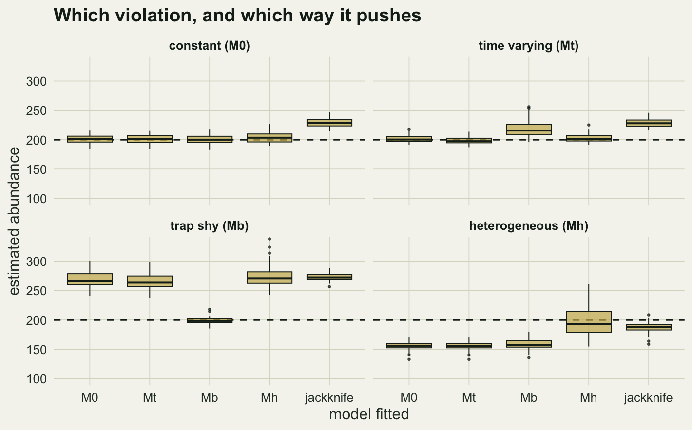
Can model selection find the right one
If the bias depends this much on which violation is present, everything rests on being able to tell them apart from the capture histories.
pick_rate <- function(r) {
  aic <- as.matrix(r[, c("aic_M0", "aic_Mt", "aic_Mb", "aic_Mh")])
  picked <- c("M0", "Mt", "Mb", "Mh")[apply(aic, 1, which.min)]
  round(100 * table(factor(picked, levels = c("M0", "Mt", "Mb", "Mh"))) / nrow(r))
}
selection <- do.call(rbind, lapply(results, pick_rate))
selection
M0 Mt Mb Mh
constant (M0) 75 7 15 3
time varying (Mt) 0 100 0 0
trap shy (Mb) 0 3 97 0
heterogeneous (Mh) 0 2 0 98It can, on data this size. The generating model has the lowest AIC in the large majority of replicates in every scenario, and the mistakes it does make are between models whose estimates are similar. Two hundred animals over six occasions with a mean capture probability of 0.30 is a generous study, and the message here is a positive one: the diagnosis is available in the data, and skipping the comparison is a choice rather than a limitation.
How much heterogeneity is too much
The Mh scenario above used one particular amount of individual variation. Holding the mean capture probability fixed and varying its spread shows how quickly the constant probability estimator gives way.
nll_two_pt <- function(par, x, n_seen) {
  N <- n_seen + exp(par[1]); w <- plogis(par[2])
  p1 <- plogis(par[3]); p2 <- plogis(par[4])
  hist_p <- function(k) log(w * p1^k * (1 - p1)^(n_occ - k) +
                              (1 - w) * p2^k * (1 - p2)^(n_occ - k))
  -(lgamma(N + 1) - lgamma(N - n_seen + 1) +
      sum(hist_p(x)) + (N - n_seen) * hist_p(0))
}
fit_hetero <- function(X) {
  s <- X[rowSums(X) > 0, , drop = FALSE]; n_seen <- nrow(s); x <- rowSums(s)
  f0 <- optim(c(log(5), 0), nll_m0, x = x, n_seen = n_seen)
  fh <- optim(c(log(5), 0, 0), nll_mh, x = x, n_seen = n_seen,
              control = list(maxit = 3000))
  f2 <- optim(c(log(5), 0, -1, 1), nll_two_pt, x = x, n_seen = n_seen,
              control = list(maxit = 5000))
  c(M0 = n_seen + exp(f0$par[1]), beta = n_seen + exp(fh$par[1]),
    two_pt = n_seen + exp(f2$par[1]),
    jackknife = n_seen + sum(x == 1) * (n_occ - 1) / n_occ,
    nll_beta = fh$value, nll_two = f2$value)
}

set.seed(21)
mean_p <- p_flat
shapes <- c(50, 6, 2.4, 1.2, 0.6)
sweep_h <- do.call(rbind, lapply(shapes, function(a) {
  b  <- a * (1 - mean_p) / mean_p
  cv <- sqrt((a * b) / ((a + b)^2 * (a + b + 1))) / mean_p
  r  <- as.data.frame(t(replicate(50, fit_hetero(gen_mh(n_true, a, b)))))
  data.frame(cv = cv, M0 = median(r$M0), beta = median(r$beta),
             two_pt = median(r$two_pt), jackknife = median(r$jackknife))
}))
print(round(sweep_h, 1))
cv M0 beta two_pt jackknife
1 0.1 197.7 200.7 200.6 225.0
2 0.3 189.4 201.6 201.2 220.8
3 0.5 172.1 196.0 183.9 203.3
4 0.7 156.8 188.7 172.3 187.9
5 0.9 134.8 198.0 151.6 163.8At a coefficient of variation of 0.33 in capture probability, which is modest for a real population, the constant probability estimate is already 5 per cent low. At 0.88 it is 33 per cent low.
The jackknife is the standard insurance against this, and the first row is its premium. On data with essentially no heterogeneity it returns 225 against a true 200, an overestimate of 12 per cent. Insurance that costs a 12 per cent bias when the risk is absent is worth buying only when the risk is real, which is an argument for looking rather than for defaulting either way.
d_sw <- do.call(rbind, lapply(c("M0", "beta", "two_pt", "jackknife"), function(k)
  data.frame(cv = sweep_h$cv, value = sweep_h[[k]], estimator = k)))
d_sw$estimator <- factor(d_sw$estimator, levels = c("M0", "beta", "two_pt", "jackknife"),
                         labels = c("M0, constant p", "Mh, beta mixture",
                                    "Mh, two point mixture", "jackknife"))

ggplot(d_sw, aes(cv, value, colour = estimator)) +
  geom_hline(yintercept = n_true, colour = te_ink, linetype = "dashed",
             linewidth = 0.6) +
  geom_line(linewidth = 1) + geom_point(size = 2.2) +
  scale_colour_manual(values = c(te_rust, te_forest, te_gold, "#7b6a4f"),
                      name = NULL) +
  labs(x = "coefficient of variation of individual capture probability",
       y = "median estimated abundance",
       title = "Where the constant probability estimate goes") +
  theme_datasheet() +
  theme(legend.position = "bottom", legend.text = element_text(size = 9))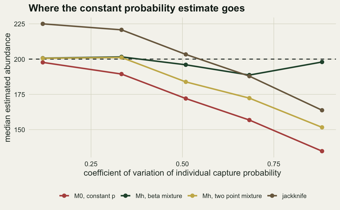
Two heterogeneity models, one dataset, two answers
The last column of that sweep is a second Mh model: instead of a beta distribution of capture probabilities it assumes two kinds of animal, easy and hard, in unknown proportions. Both are respectable choices, and on the same data they do not agree.
set.seed(404)
pair <- as.data.frame(t(replicate(40, fit_hetero(gen_mh(n_true, 1.2, 2.8)))))
gap_n   <- median(abs(pair$beta - pair$two_pt))
gap_nll <- median(abs(pair$nll_beta - pair$nll_two))
Over 40 datasets the two mixing distributions differ by a median of 27 animals, which is 13 per cent of the true abundance, while their log likelihoods differ by a median of 0.73. The data cannot separate them and the answers are not the same. Link proved in 2003 that this is not a numerical accident: different mixing distributions can give identical probabilities for every observable capture frequency and still imply different numbers of animals never caught. The unseen part of the population is where the disagreement lives, and no amount of fieldwork on the seen part settles it.
ggplot(pair, aes(beta, two_pt)) +
  geom_abline(slope = 1, intercept = 0, colour = te_ink, linetype = "dashed",
              linewidth = 0.6) +
  geom_hline(yintercept = n_true, colour = te_gold, linewidth = 0.7) +
  geom_vline(xintercept = n_true, colour = te_gold, linewidth = 0.7) +
  geom_point(colour = te_forest, size = 2.2, alpha = 0.85) +
  labs(x = "abundance from the beta mixture",
       y = "abundance from the two point mixture",
       title = "Same histories, two defensible answers") +
  theme_datasheet()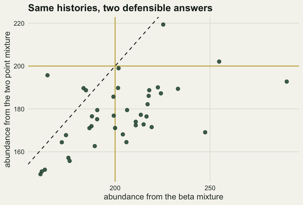
What to report
Fit more than M0 and report the comparison. The measurement above says the diagnosis is available in a study of ordinary size, so a paper that reports only M0 has declined to look rather than been unable to.
Say which direction the residual risk runs. A trap response and individual heterogeneity bias abundance in opposite directions, so a study that has ruled out one of them has not narrowed the interval on the other.
Report the number of animals caught exactly once alongside the estimate. It is the statistic every heterogeneity correction is built from, and a reader can see from it how much of the answer is extrapolation.
If a heterogeneity model is used, say which mixing distribution and acknowledge that the choice moves the answer. Reporting a beta mixture estimate to three significant figures without that sentence overstates what the data contain.
Honest limits
The population is genuinely closed here: no births, no deaths, no movement in or out. Real six occasion studies are closed by assumption and the assumption is usually a compromise about the length of the trapping session. Losses to the population and a trap response are also hard to tell apart from capture histories alone.
Only one violation acts at a time. The named combinations Mth, Mbh and Mtbh exist because real studies have several at once, and the biases do not simply add: a trap response pushing up and heterogeneity pulling down can cancel in the estimate while leaving the interval far too narrow.
The behavioural response modelled is trap shyness, where recapture is less likely than first capture. Trap happiness is at least as common with baited traps and reverses the sign, so the direction reported above for Mb is the direction of that particular scenario, not a property of behavioural response as such.
The two hundred animals and mean capture probability of 0.30 make this a well sampled study. Halve the capture probability and the number of animals never seen grows, every estimator’s variance grows with it, and the model selection result reported here would not survive.
There is a reconciliation to make with the mark resight post on this site, where individual heterogeneity did not bias the point estimate and instead destroyed the coverage of the interval. The difference is structural. In mark resight the number of marked animals is known, so heterogeneity affects how well the marked fraction is estimated. Here abundance is inferred from the shape of the capture frequency distribution, and heterogeneity changes that shape, so it moves the estimate itself.
References
Burnham KP, Overton WS 1978 Biometrika 65(3):625-633 (10.1093/biomet/65.3.625)
Pledger S 2000 Biometrics 56(2):434-442 (10.1111/j.0006-341X.2000.00434.x)
Link WA 2003 Biometrics 59(4):1123-1130 (10.1111/j.0006-341X.2003.00129.x)