library(ggplot2)
library(patchwork)

te_paper  <- "#f5f4ee"
te_ink    <- "#16241d"
te_body   <- "#2c3a31"
te_forest <- "#275139"
te_rust   <- "#b5534e"
te_gold   <- "#c9b458"
te_line   <- "#dad9ca"

theme_datasheet <- function() {
  theme_minimal(base_size = 12) +
    theme(plot.background  = element_rect(fill = te_paper, colour = NA),
          panel.background = element_rect(fill = te_paper, colour = NA),
          panel.grid.major = element_line(colour = te_line, linewidth = 0.3),
          panel.grid.minor = element_blank(),
          text             = element_text(colour = te_body),
          plot.title       = element_text(colour = te_ink, face = "bold"),
          plot.subtitle    = element_text(colour = te_body),
          axis.text        = element_text(colour = te_body))
}Declaring eradication after empty traps
R
eradication
invasive species
removal sampling
detection
simulation
ecology tutorial
A run of empty trap sessions sized from the removal capture rate is calibrated only when every animal is equally catchable. Testing eradication rules in R.
An island rat eradication has reached the stage where the traps come back empty. The first nights took dozens of animals, the catch fell away over a few weeks, and now session after session produces nothing. Someone has to write the sentence that the island is clear, and the sentence needs a number behind it. The usual reasoning goes like this: the removal series itself says how catchable a rat is, so work out how many empty sessions in a row a surviving rat would have had only a five per cent chance of slipping through, and stop when the run of empty sessions is that long.
That rule is a stylised version of what programmes do. Real eradications also run independent surveillance with its own detection probability (chew cards, cameras, dogs, bait stations) and many now report a formal probability of eradication built from those data, as Ramsey, Parkes and Morrison did for feral pigs on Santa Cruz Island. Rout, Salomon and McCarthy set out how to trade the cost of more searching against the cost of declaring too early. The simple rule is still worth measuring, because the arithmetic inside it is the arithmetic inside the more elaborate versions: a detection probability estimated from the animals already found is applied to the animals not found.
The rule is correct if every animal is equally catchable, and this post checks it in closed form for that case. It then gives the animals different capture probabilities around the same mean and measures what happens to the declaration. Removal is a filter: the catchable animals are caught first, so the population left behind is less catchable than the one the capture rate was estimated from, and the gap grows exactly when the programme is deciding whether to stop.
Several posts on this site sit next to this one without covering it. How many visits? Occupancy survey design turns 1 - (1 - p)^K into the number of visits before a run of blanks is good evidence of absence, with one detection probability shared by every site. Removal and depletion sampling in R fits the Zippin model and says in prose that every animal must have the same catch probability on every pass; it does not run the heterogeneous case. Capture heterogeneity: Mt, Mb and Mh in R shows heterogeneity pulling a closed capture-recapture abundance estimate below the truth. Here the same heterogeneity becomes a decision error rather than a biased estimate. Checking a sequential decision model finds a permanent eradication that is an artefact of a coarse state grid; that is a modelling problem in a decision model, not a detection problem in the field data.
The rule and the machinery
A closed population of 80 animals is trapped in sessions. Every animal still present is caught and removed in a session with its own probability, independently of the others, so the session in which an animal is caught is a geometric waiting time. The programme sees only the catch per session. After every empty session it refits the capture probability from the catches so far and computes the run length that a single survivor at that probability would have escaped with probability five per cent,
\[k = \left\lceil \frac{\log 0.05}{\log(1 - \hat p)} \right\rceil ,\]
and it declares eradication at the first empty session that ends a run of at least k empty sessions. A run that never qualifies within 300 sessions is stopped and counted as capped, not as a declaration.
The capture probability is the conditional removal estimate. Given that T animals were caught in the first s sessions, their capture sessions follow a geometric distribution truncated at s, so the likelihood depends on p alone and N drops out. This is the conditional form of the Zippin likelihood; the score equation is monotone in p, which lets the fit run as a bisection over every run and every session at once instead of one optimize call at a time.
n0     <- 80
p_mean <- 0.3
cap    <- 300
alpha  <- 0.05

sim_cell <- function(phi, n_run) {
  p_ind <- if (is.infinite(phi)) matrix(p_mean, n_run, n0) else
    matrix(rbeta(n_run * n0, p_mean * phi, (1 - p_mean) * phi), n_run, n0)
  list(p = p_ind, t = matrix(rgeom(n_run * n0, p_ind) + 1, n_run, n0))
}

catch_mat <- function(t_cap) {
  t(apply(t_cap, 1, function(v) tabulate(v[v <= cap], nbins = cap)))
}
sess_mat <- function(n_row) matrix(seq_len(cap), n_row, cap, byrow = TRUE)

cond_nll <- function(p, x_s, s) {
  j_s <- seq_len(s)
  tot <- sum(x_s)
  -(tot * log(p) + sum(x_s * (j_s - 1)) * log(1 - p) -
      tot * log(1 - (1 - p)^s))
}

phat_mat <- function(x) {
  s_mat <- sess_mat(nrow(x))
  tot   <- t(apply(x, 1, cumsum))
  wsum  <- t(apply(x * (s_mat - 1), 1, cumsum))
  lo <- matrix(1e-6, nrow(x), cap)
  hi <- matrix(1 - 1e-6, nrow(x), cap)
  for (it in 1:45) {
    mid <- (lo + hi) / 2
    q_m <- 1 - mid
    up  <- tot / mid - wsum / q_m - tot * s_mat * q_m^(s_mat - 1) / (1 - q_m^s_mat) > 0
    lo[up]  <- mid[up]
    hi[!up] <- mid[!up]
  }
  (lo + hi) / 2
}

run_len <- function(x) {
  s_mat <- sess_mat(nrow(x))
  s_mat - t(apply(s_mat * (x > 0), 1, cummax))
}

declare <- function(x, rl, kk, t_cap) {
  dmat  <- (x == 0) & (rl >= kk)
  hit   <- rowSums(dmat) > 0
  s_dec <- ifelse(hit, max.col(dmat, ties.method = "first"), cap)
  data.frame(s = s_dec, surv = rowSums(t_cap > s_dec), capped = !hit)
}

k_of <- function(p) ceiling(log(alpha) / log(1 - p))set.seed(4021)
chk_cell <- sim_cell(5, 20)
chk_x <- catch_mat(chk_cell$t)
chk_ph <- phat_mat(chk_x)
chk_s <- sample(30:120, 20)
chk_opt <- vapply(seq_len(20), function(i) {
optimize(cond_nll, c(1e-6, 1 - 1e-6), x_s = chk_x[i, seq_len(chk_s[i])],
s = chk_s[i], tol = 1e-10)$minimum
}, 0)
chk_gap <- max(abs(chk_opt - chk_ph[cbind(seq_len(20), chk_s)]))The bisection was checked against optimize on the same conditional likelihood for twenty random run and session pairs; the largest difference in the estimated capture probability was 4.93e-09.
With equal catchability the rule has an exact answer
If every animal has the same known p, the whole programme is a Markov chain on the number of animals left and the length of the current empty run, and the probability that it declares with survivors has a short recursion. Write f(n) for that probability starting from n animals at the start of a run, and q = 1 - p. From n animals a session is empty with probability q^n. The run either reaches k empty sessions before any capture, which is a false declaration, or a capture of c animals restarts the run from n - c. Summing the geometric series over the run positions gives
\[f(n) = q^{nk} + \frac{1 - q^{nk}}{1 - q^n} \sum_{c=1}^{n} \binom{n}{c} p^c q^{n-c} f(n-c), \qquad f(0) = 0 .\]
For a single animal f(1) = q^k, which is the five per cent bound the rule was built on. For eighty animals the chain has many chances to fall into a long empty run while animals remain, but each of those runs has to beat q^{nk} with n of at least one, so the answer is not obvious in advance.
exact_fail <- function(p, k, n_start) {
  q_p <- 1 - p
  f_n <- numeric(n_start + 1)
  for (n in seq_len(n_start)) {
    c_s  <- seq_len(n)
    a_n  <- sum(dbinom(c_s, n, p) * f_n[n - c_s + 1])
    f_n[n + 1] <- q_p^(n * k) + a_n * (1 - q_p^(n * k)) / (1 - q_p^n)
  }
  f_n[n_start + 1]
}

k_mean     <- k_of(p_mean)
one_surv   <- (1 - p_mean)^k_mean
exact_mean <- exact_fail(p_mean, k_mean, n0)

p_grid  <- seq(0.05, 0.6, by = 0.01)
exact_df <- data.frame(p = p_grid,
                       programme = vapply(p_grid, function(p) exact_fail(p, k_of(p), n0), 0),
                       single = (1 - p_grid)^k_of(p_grid))

n_known <- 20000
set.seed(7730)
known_t   <- matrix(rgeom(n_known * n0, p_mean) + 1, n_known, n0)
known_x   <- catch_mat(known_t)
known_dec <- declare(known_x, run_len(known_x), k_mean, known_t)
known_rate <- mean(known_dec$surv > 0)
known_se   <- sqrt(known_rate * (1 - known_rate) / n_known)
known_z    <- (known_rate - exact_mean) / known_se
At p = 0.3 the rule asks for 9 empty sessions, and a single survivor escapes that many with probability 0.0404; the rounding up of k puts this below five per cent. The recursion gives a probability of 0.0351 that the programme declares with at least one animal left. A simulation of 20000 programmes with the known p returns 0.0348 with a Monte Carlo standard error of 0.0013, which is -0.2 standard errors from the exact value. The simulator and the recursion agree, and with a known, shared p the rule does what it promises.
p_check <- c(0.1, 0.3, 0.5)
n_phat  <- 3000
set.seed(8124)
phat_homog <- do.call(rbind, lapply(p_check, function(p) {
  t_cap <- matrix(rgeom(n_phat * n0, p) + 1, n_phat, n0)
  x     <- catch_mat(t_cap)
  ph    <- phat_mat(x)
  d_out <- declare(x, run_len(x), k_of(ph), t_cap)
  rate  <- mean(d_out$surv > 0 & !d_out$capped)
  data.frame(p = p, rate = rate, se = sqrt(rate * (1 - rate) / n_phat),
             exact = exact_fail(p, k_of(p), n0), capped = mean(d_out$capped))
}))
ph_mid <- phat_homog[phat_homog$p == p_mean, ]
The programme does not know p; it estimates it. With the estimate refitted after every empty session, 3000 programmes at p = 0.3 declare with a survivor in 0.0477 of runs (standard error 0.0039), against 0.0351 with p known. At p = 0.1 the rates are 0.0633 estimated and 0.0467 exact, and at 0.5 they are 0.0317 and 0.0231. The capped share is 0.000 in all three. Estimating p does cost something: at p = 0.3 the false declaration rate is 3.2 standard errors above the known-p value, and at p = 0.1 it passes the nominal five per cent. The reason is that k is rounded from an estimate that is sometimes too high, and a single high estimate at the right moment is enough to stop. That cost is small next to what follows, and the rule is close to its promise in the world it assumes.
exact_long <- rbind(
  data.frame(p = exact_df$p, value = exact_df$single, what = "one survivor escapes k sessions"),
  data.frame(p = exact_df$p, value = exact_df$programme, what = "programme of 80 declares with survivors"))

ggplot(exact_long, aes(p, value, colour = what)) +
  geom_hline(yintercept = alpha, linetype = "dashed", colour = te_body, linewidth = 0.5) +
  geom_line(linewidth = 0.8) +
  geom_errorbar(data = phat_homog, aes(x = p, ymin = rate - 1.96 * se, ymax = rate + 1.96 * se),
                inherit.aes = FALSE, width = 0.012, colour = te_rust, linewidth = 0.6) +
  geom_point(data = phat_homog, aes(p, rate), inherit.aes = FALSE,
             colour = te_rust, size = 2.4) +
  scale_colour_manual(values = c(te_gold, te_forest), name = NULL) +
  coord_cartesian(ylim = c(0, 0.08)) +
  labs(x = "capture probability per session (same for every animal)",
       y = "probability of a false declaration",
       title = "Equal catchability: close to the promise",
       subtitle = "red points: capture probability estimated from the removal series") +
  theme_datasheet() +
  theme(legend.position = "bottom")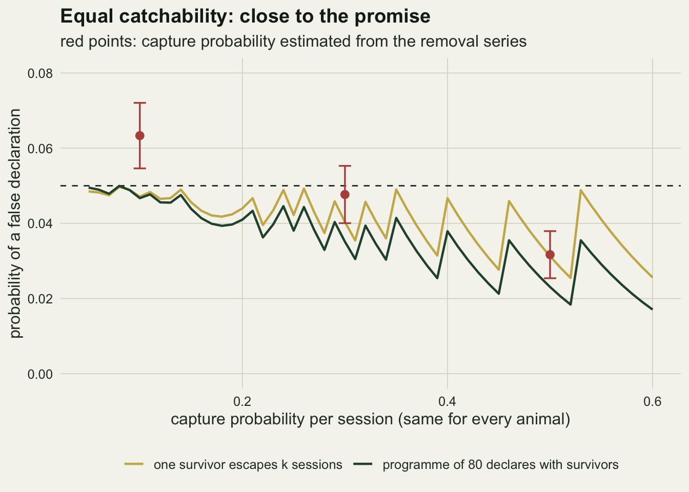
The same mean, different animals
Now let each animal draw its own capture probability from a beta distribution with mean 0.3 and precision phi, so that the variance is 0.3 * 0.7 / (1 + phi). Infinite precision is the equal catchability case above; a precision of 20 is mild variation, 5 is the kind of spread that trap-shy and trap-happy individuals produce, and 1.5 puts a large share of the population below one catch in twenty sessions. The design values and the 1000 runs per cell were fixed before the simulation was run.
phi_grid <- c(Inf, 20, 5, 1.5)
phi_lab  <- c("equal", "20", "5", "1.5")
n_het    <- 1000
extras   <- c(0, 5, 10, 20, 40, 80, 160)

set.seed(5561)
het <- lapply(phi_grid, function(phi) {
  cell <- sim_cell(phi, n_het)
  x    <- catch_mat(cell$t)
  ph   <- phat_mat(x)
  rl   <- run_len(x)
  kk   <- k_of(ph)
  d0   <- declare(x, rl, kk, cell$t)
  bad  <- which(d0$surv > 0 & !d0$capped)
  ok   <- which(!d0$capped)
  surv_p <- vapply(bad, function(i) mean(cell$p[i, cell$t[i, ] > d0$s[i]]), 0)
  sweep_e <- do.call(rbind, lapply(extras, function(e) {
    d_e <- declare(x, rl, kk + e, cell$t)
    data.frame(extra = e, fail = mean(d_e$surv > 0 & !d_e$capped),
               capped = mean(d_e$capped), med_s = median(d_e$s))
  }))
  traj <- apply(ph[, 1:60], 2, median)
  list(d0 = d0, fail = mean(d0$surv > 0 & !d0$capped), capped = mean(d0$capped),
       surv_bad = mean(d0$surv[bad]), med_s = median(d0$s[ok]),
       ph_dec = ph[cbind(ok, d0$s[ok])], k_dec = kk[cbind(ok, d0$s[ok])],
       surv_p = surv_p, sweep = sweep_e, traj = traj)
})

het_tab <- data.frame(
  phi = phi_lab,
  fail = vapply(het, `[[`, 0, "fail"),
  capped = vapply(het, `[[`, 0, "capped"),
  surv_bad = vapply(het, `[[`, 0, "surv_bad"),
  med_s = vapply(het, `[[`, 0, "med_s"),
  ph_med = vapply(het, function(h) median(h$ph_dec), 0),
  k_med = vapply(het, function(h) median(h$k_dec), 0),
  surv_p = vapply(het, function(h) if (length(h$surv_p)) mean(h$surv_p) else NA_real_, 0))
het_tab$se <- sqrt(het_tab$fail * (1 - het_tab$fail) / n_het)
het_tab$phi <- factor(het_tab$phi, levels = phi_lab)
With equal catchability the refitted rule declares with survivors in 0.048 of 1000 runs (standard error 0.007). At the same mean capture probability, a precision of 20 raises that to 0.249 (standard error 0.014), a precision of 5 to 0.798 and a precision of 1.5 to 0.993, with 0.007 of runs in that last cell reaching the cap without a declaration; in the other three cells the largest capped share is 0.000.
The failures are not a single straggler. When the programme declares wrongly it leaves on average 1.02 animals with equal catchability, 2.39 at precision 5 and 11.2 at precision 1.5, which on an island is a breeding population. The programme does notice something: the median session of declaration moves from 23 to 43 and 70, and the median k at declaration from 9 to 14 and 20. It stops anyway.
p_fail <- ggplot(het_tab, aes(phi, fail)) +
  geom_hline(yintercept = alpha, linetype = "dashed", colour = te_body, linewidth = 0.5) +
  geom_col(fill = te_rust, width = 0.6) +
  geom_errorbar(aes(ymin = fail - 1.96 * se, ymax = fail + 1.96 * se),
                width = 0.15, colour = te_ink, linewidth = 0.5) +
  scale_y_continuous(limits = c(0, 1)) +
  labs(x = "precision of individual catchability", y = "declared with survivors",
       title = "False declarations")

ph_bad <- do.call(rbind, lapply(seq_along(het)[-1], function(i) {
  h   <- het[[i]]
  bad <- which(h$d0$surv > 0 & !h$d0$capped)
  ok  <- which(!h$d0$capped)
  data.frame(phi = phi_lab[i], estimate = h$ph_dec[match(bad, ok)], survivors = h$surv_p)
}))
ph_bad$phi <- factor(ph_bad$phi, levels = phi_lab[-1])

p_gap <- ggplot(ph_bad, aes(estimate, survivors, colour = phi)) +
  geom_abline(slope = 1, intercept = 0, linetype = "dashed", colour = te_body, linewidth = 0.5) +
  geom_point(alpha = 0.45, size = 1.1) +
  scale_colour_manual(values = c(te_gold, te_forest, te_rust), name = "precision") +
  coord_cartesian(xlim = c(0, 0.5), ylim = c(0, 0.5)) +
  labs(x = "estimated capture probability", y = "mean p of the animals left",
       title = "Estimate against survivors") +
  theme(legend.position = "bottom")

(p_fail + theme_datasheet()) + (p_gap + theme_datasheet() + theme(legend.position = "bottom")) +
  plot_annotation(theme = theme_datasheet())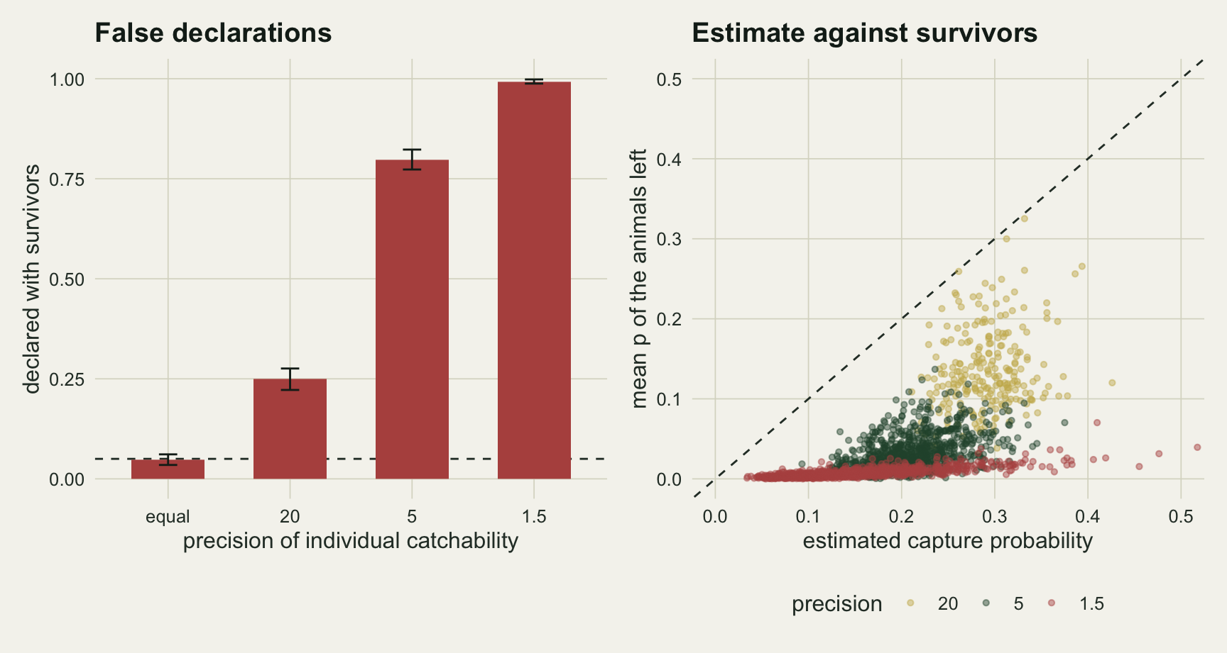
The right panel is the mechanism in one picture. In the wrongly declared programmes at precision 5, the median estimated capture probability at declaration is 0.210, while the animals still on the island have a mean capture probability of 0.034. The rule sizes k for a survivor that is roughly 6 times more catchable than the survivors it has left behind.
Removal is a filter
The size of that gap does not need a simulation. If capture probabilities follow a beta distribution with shape parameters a and b, an animal that has escaped s sessions has survived s independent Bernoulli trials with failure probability 1 - p, so its capture probability has the beta posterior with parameters a and b + s. The mean capture probability of the animals still present after s sessions is therefore a / (a + b + s), whatever happened to the catch. The estimate the programme uses is pooled over the animals caught so far, most of which were caught early.
set.seed(6109)
filt <- do.call(rbind, lapply(phi_grid[-1], function(phi) {
  a_s   <- p_mean * phi
  b_s   <- (1 - p_mean) * phi
  cell  <- sim_cell(phi, 2000)
  s_seq <- 1:60
  sim_m <- vapply(s_seq, function(s) mean(cell$p[cell$t > s]), 0)
  data.frame(phi = as.character(phi), s = s_seq, closed = a_s / (a_s + b_s + s_seq),
             simulated = sim_m, phat = het[[which(phi_grid == phi)]]$traj)
}))
filt$phi <- factor(filt$phi, levels = phi_lab[-1])
filt_gap <- max(abs(filt$closed - filt$simulated))
at_40    <- filt[filt$s == 40 & filt$phi == "5", ]
Across the three heterogeneous cells and the first 60 sessions, the closed form and the simulated mean capture probability of the animals still present differ by at most 0.0056. At precision 5 and session 40 the animals left have a mean capture probability of 0.033, and the median estimate in the programmes at that session is 0.202.
ggplot(filt, aes(s)) +
  geom_line(aes(y = closed, colour = phi), linewidth = 0.8) +
  geom_point(data = filt[filt$s %% 5 == 0, ], aes(y = simulated, colour = phi), size = 1.6) +
  geom_line(data = filt[filt$s >= 5, ], aes(y = phat, colour = phi),
            linetype = "dashed", linewidth = 0.7) +
  scale_colour_manual(values = c(te_gold, te_forest, te_rust), name = "precision") +
  coord_cartesian(ylim = c(0, 0.45)) +
  labs(x = "session", y = "capture probability",
       title = "The animals left are not the animals caught",
       subtitle = "solid: animals still present; dashed: removal estimate (median over runs)") +
  theme_datasheet() +
  theme(legend.position = "bottom")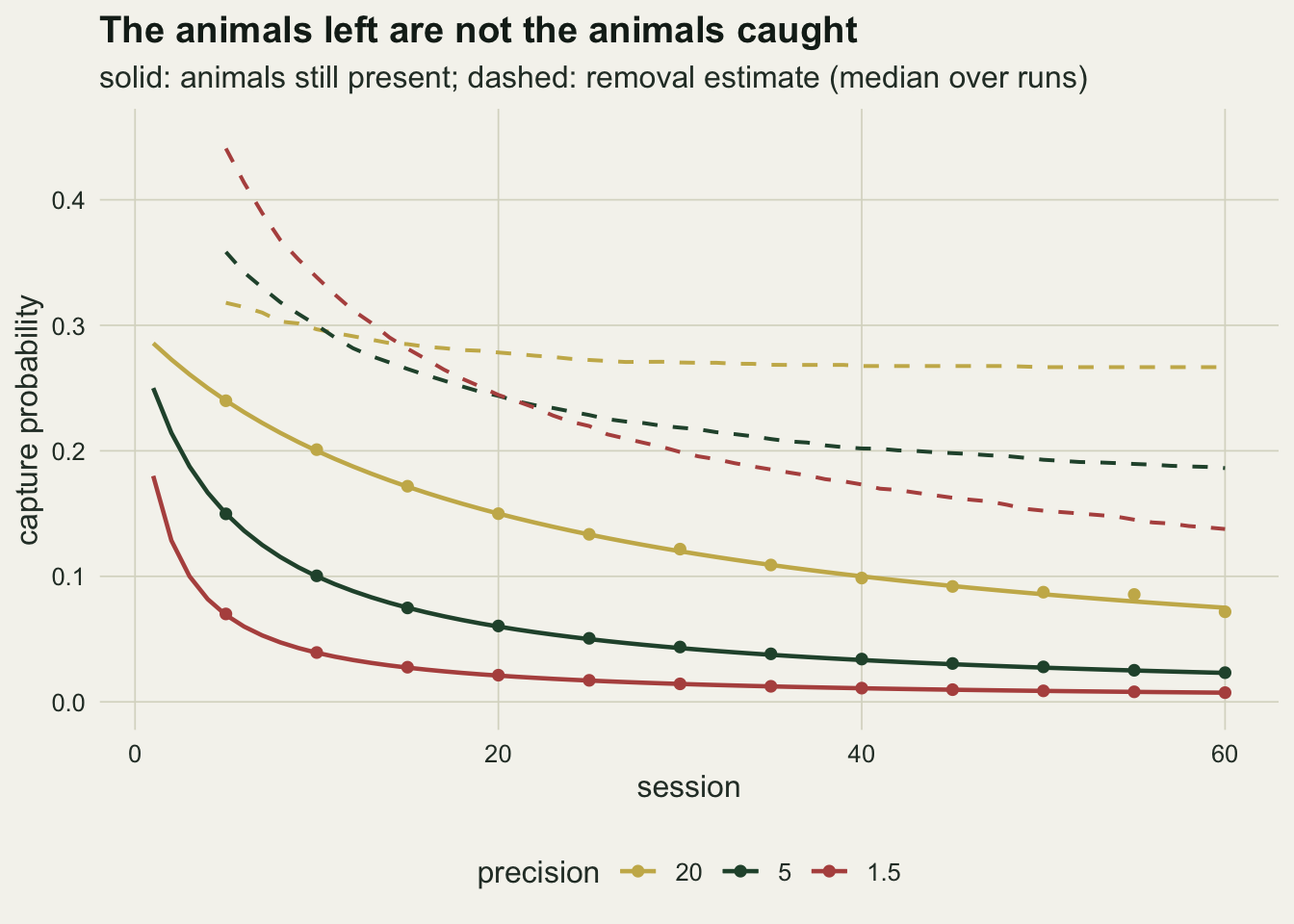
What more empty sessions buy
The obvious fix is to demand more. The sweep below adds a fixed number of empty sessions to k and reruns the declaration on the same simulated programmes, so the only thing that changes is the rule.
sweep_all <- do.call(rbind, lapply(seq_along(het), function(i) {
  cbind(phi = phi_lab[i], het[[i]]$sweep)
}))
sweep_all$phi <- factor(sweep_all$phi, levels = phi_lab)
sweep_all$cond <- ifelse(sweep_all$capped < 1, sweep_all$fail / (1 - sweep_all$capped), NA_real_)

first_ok <- function(sw) {
  hit <- sw$extra[sw$fail <= alpha]
  if (length(hit)) min(hit) else NA
}
need_20 <- first_ok(sweep_all[sweep_all$phi == "20", ])
row_20  <- sweep_all[sweep_all$phi == "20" & sweep_all$extra == need_20, ]
row_5   <- sweep_all[sweep_all$phi == "5" & sweep_all$extra == max(extras), ]
row_15  <- sweep_all[sweep_all$phi == "1.5" & sweep_all$extra == max(extras), ]
cond_15_min <- min(sweep_all$cond[sweep_all$phi == "1.5"], na.rm = TRUE)

surv_any <- function(phi, s) {
  if (is.infinite(phi)) return(1 - (1 - (1 - p_mean)^s)^n0)
  a_s <- p_mean * phi
  b_s <- (1 - p_mean) * phi
  1 - (1 - exp(lbeta(a_s, b_s + s) - lbeta(a_s, b_s)))^n0
}
oracle_s <- vapply(phi_grid, function(phi) {
  ceiling(uniroot(function(ls) surv_any(phi, exp(ls)) - alpha,
                  c(0, 30), tol = 1e-9)$root |> exp())
}, 0)
At precision 20 adding 20 empty sessions brings the false declaration rate to 0.022, at a median programme length of 51 sessions; the capped share is 0.000, and 0.022 of the declarations that are made leave animals behind. At precision 5 even 160 extra empty sessions leave 0.118 of all programmes declaring with survivors, and 0.239 never declare within 300 sessions. Counted among the programmes that do declare, the wrong share is 0.155, which is the number a manager reading one declaration should care about. At precision 1.5 the same addition gives 0.043 of all programmes declaring with survivors only because 0.957 of programmes hit the cap: the declarations that are made leave animals behind in 1.000 of cases, and the lowest that share reaches anywhere in the sweep is 0.9946. Extra sessions at that precision do not make a declaration trustworthy; they only make it rarer.
There is a cleaner way to see the cost. If the beta distribution were known, the probability that at least one of the 80 animals is still present after s sessions is 1 - (1 - S(s))^80, where S(s) = B(a, b + s) / B(a, b) is the chance that one animal escapes s sessions. Setting that to five per cent gives the session at which a declaration would be honest, with no data used at all: 21 sessions with equal catchability, 40 at precision 20, 499 at precision 5 and 10,122,303 at precision 1.5. With equal catchability the escape probability falls geometrically; with a beta distribution it falls only as a power of s, because the least catchable animals are the ones that remain.
sweep_long <- rbind(
  data.frame(sweep_all[, c("phi", "extra")], panel = "all programmes: declared with survivors", value = sweep_all$fail),
  data.frame(sweep_all[, c("phi", "extra")], panel = "declarations made with survivors", value = sweep_all$cond),
  data.frame(sweep_all[, c("phi", "extra")], panel = "no declaration by 300", value = sweep_all$capped))
sweep_long$panel <- factor(sweep_long$panel, levels = unique(sweep_long$panel))
sweep_long <- sweep_long[!is.na(sweep_long$value), ]

ggplot(sweep_long, aes(extra, value, colour = phi)) +
  geom_hline(data = data.frame(panel = levels(sweep_long$panel)[1:2], y = alpha),
             aes(yintercept = y), linetype = "dashed", colour = te_body, linewidth = 0.5) +
  geom_line(linewidth = 0.8) +
  geom_point(size = 1.8) +
  facet_wrap(~ panel) +
  scale_colour_manual(values = c(te_ink, te_gold, te_forest, te_rust), name = "precision") +
  scale_x_continuous(breaks = c(0, 40, 80, 160)) +
  scale_y_continuous(limits = c(0, 1)) +
  labs(x = "extra empty sessions demanded beyond k",
       y = "share",
       title = "Paying in sessions",
       subtitle = "the same simulated programmes under each rule") +
  theme_datasheet() +
  theme(legend.position = "bottom",
        strip.text = element_text(colour = te_ink, face = "bold"))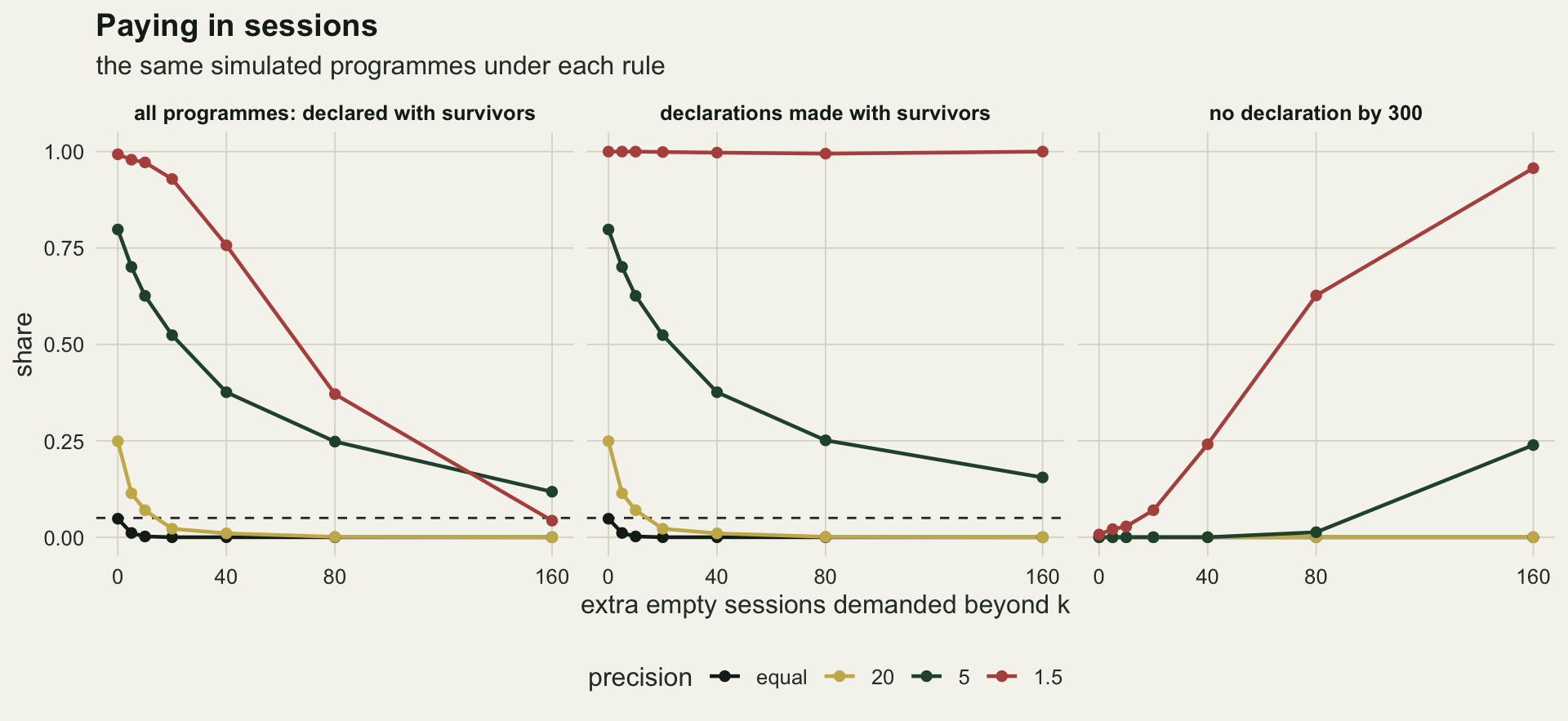
Fitting the heterogeneity from the same series
The sweep and the oracle both use knowledge the programme does not have. The operational repair is to fit a heterogeneous model to the removal series and declare only when the model’s own estimate of what is left is small. The beta distribution of capture probability gives the beta-geometric model for the capture session: the probability of capture in session j is B(a + 1, b + j - 1) / B(a, b). Conditioning on capture by session s again removes N, the two shape parameters are fitted by optim on the log scale, and the estimated number of animals left is T S(s) / (1 - S(s)). The repaired rule declares at an empty session when that estimate is at most -log(0.95), which is a five per cent chance of any survivor if the count left is Poisson.
This is the most favourable repair available, because the fitted model is the model that generated the data. Whether two shape parameters are identifiable from one series of eighty capture sessions is a separate question, and the chunk counts fits that end on a bound of the parameter box (a log shape of 7 means the fit has decided the animals are alike), records the fitted precision a + b of the last fit, and counts the fits where optim reports non-convergence. A fitted precision above 100, five times the mildest true value, is read as a fit that sees no heterogeneity; that threshold was set before the arm was run. It is refitted at every empty session, which is slow, so this arm uses 300 runs per cell.
bg_fit <- function(x, s, start) {
  j_s <- which(x[seq_len(s)] > 0)
  x_j <- x[j_s]
  tot <- sum(x_j)
  nll <- function(th) {
    a_s <- exp(th[1]); b_s <- exp(th[2]); lb <- lbeta(a_s, b_s)
    -(sum(x_j * (lbeta(a_s + 1, b_s + j_s - 1) - lb)) -
        tot * log1p(-exp(lbeta(a_s, b_s + s) - lb)))
  }
  o_fit <- optim(start, nll, method = "L-BFGS-B", lower = c(-7, -7), upper = c(7, 9))
  a_s <- exp(o_fit$par[1]); b_s <- exp(o_fit$par[2])
  s_esc <- exp(lbeta(a_s, b_s + s) - lbeta(a_s, b_s))
  list(par = o_fit$par, left = tot * s_esc / (1 - s_esc), conv = o_fit$convergence)
}

n_rep <- 300
set.seed(9357)
repair <- do.call(rbind, lapply(seq_along(phi_grid), function(i) {
  cell <- sim_cell(phi_grid[i], n_rep)
  x    <- catch_mat(cell$t)
  out  <- t(vapply(seq_len(n_rep), function(r) {
    st <- c(0, 0.8); n_fit <- 0; n_conv <- 0; last_par <- c(NA, NA)
    for (s in seq_len(cap)) if (x[r, s] == 0) {
      fit <- bg_fit(x[r, ], s, st)
      st <- fit$par; last_par <- fit$par
      n_fit <- n_fit + 1; n_conv <- n_conv + (fit$conv != 0)
      if (fit$left <= -log(0.95)) return(c(s, sum(cell$t[r, ] > s), 0, n_fit, n_conv, last_par))
    }
    c(cap, sum(cell$t[r, ] > cap), 1, n_fit, n_conv, last_par)
  }, numeric(7)))
  data.frame(phi = phi_lab[i], s = out[, 1], surv = out[, 2], capped = out[, 3] == 1,
             n_fit = out[, 4], n_conv = out[, 5], log_a = out[, 6],
             prec_hat = exp(out[, 6]) + exp(out[, 7]))
}))
repair$phi <- factor(repair$phi, levels = phi_lab)

rep_tab <- do.call(rbind, lapply(split(repair, repair$phi), function(d) {
  fail <- mean(d$surv > 0 & !d$capped)
  data.frame(phi = d$phi[1], fail = fail, se = sqrt(fail * (1 - fail) / nrow(d)),
             capped = mean(d$capped), med_s = median(d$s[!d$capped]),
             at_bound = mean(d$log_a >= 7 - 1e-3),
             prec_med = median(d$prec_hat), prec_big = mean(d$prec_hat > 100),
             conv_bad = sum(d$n_conv), fits = sum(d$n_fit))
}))
rep_tab$n_dec <- round((1 - rep_tab$capped) * n_rep)
rep_tab$cond  <- ifelse(rep_tab$n_dec > 0, rep_tab$fail / (1 - rep_tab$capped), NA_real_)
tot_fits <- sum(rep_tab$fits)
tot_conv <- sum(rep_tab$conv_bad)
With equal catchability the repaired rule declares with survivors in 0.057 of 300 runs (standard error 0.013), at a median session of 22; 0.737 of the final fits have a fitted precision above 100, and 0.513 sit on the bound of the shape parameter. The rest see some heterogeneity that is not there.
At precision 20 the median fitted precision is 31.3 against a true 20, and 0.337 of the final fits see no heterogeneity by the threshold above. The false declaration rate is 0.170 (standard error 0.022), against 0.249 for the original rule. Two parameters can be fitted from one removal series of eighty animals, but the series says little about the slow tail of the beta distribution, and a fit that understates the spread makes that tail too thin and declares too early.
At precision 5 the fit recovers the spread well, with a median fitted precision of 5.5, and its answer is mostly to refuse: 0.543 of programmes reach 300 sessions without a declaration, and 0.197 (standard error 0.023) of all programmes declare with survivors, against 0.798 under the original rule. That comparison flatters the repair, because its denominator includes the programmes that never declare: of the declarations the repaired rule does make at precision 5, 0.431 leave animals behind, against 0.170 at precision 20 and 0.057 with equal catchability. At precision 1.5 the capped share is 0.997, and the single declaration made in 300 runs left animals behind. Over all 157509 fits, optim reported non-convergence 1046 times, 923 of them in the precision 1.5 cell, where most fits are made on long series of empty sessions. The repair does not buy calibration at a modest extra cost. Where the heterogeneity is mild it is still miscalibrated, and where it is strong it turns false declarations into programmes that do not end, consistent with the data-free oracle sessions in the previous section (499 at precision 5 and more at precision 1.5).
outcome_of <- function(surv, capped) {
  factor(ifelse(capped, "no declaration by 300", ifelse(surv > 0, "declared, animals left", "declared, clear")),
         levels = c("declared, clear", "declared, animals left", "no declaration by 300"))
}
out_rule <- do.call(rbind, lapply(seq_along(het), function(i) {
  d <- het[[i]]$d0
  data.frame(phi = phi_lab[i], rule = "k empty sessions", outcome = outcome_of(d$surv, d$capped))
}))
out_rep <- data.frame(phi = as.character(repair$phi), rule = "beta-geometric fit",
                      outcome = outcome_of(repair$surv, repair$capped))
out_all <- rbind(out_rule, out_rep)
out_all$phi  <- factor(out_all$phi, levels = phi_lab)
out_all$rule <- factor(out_all$rule, levels = c("k empty sessions", "beta-geometric fit"))

ggplot(out_all, aes(phi, fill = outcome)) +
  geom_bar(position = "fill", width = 0.7) +
  facet_wrap(~ rule) +
  scale_fill_manual(values = c(te_forest, te_rust, te_gold), name = NULL) +
  labs(x = "precision of individual catchability", y = "share of programmes",
       title = "The repair trades false declarations for no declaration") +
  theme_datasheet() +
  theme(legend.position = "bottom",
        strip.text = element_text(colour = te_ink, face = "bold"))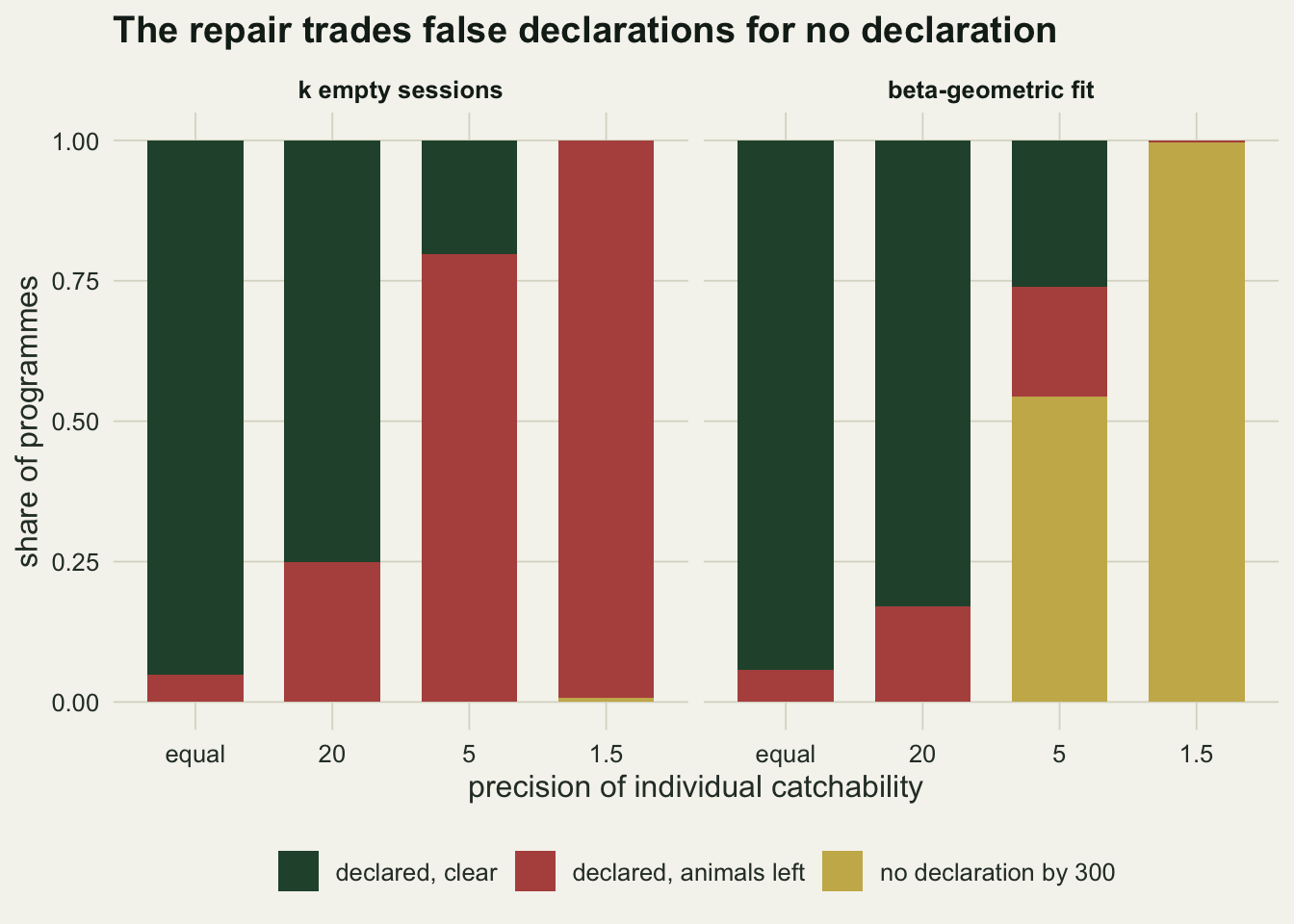
What to report
Report the rule and the capture probability it used, and say where that probability came from. A declaration that rests on a removal estimate rests on the animals that were caught, and the reader needs to know that before reading the five per cent.
Report the evidence that the animals were equally catchable, and treat its absence as a limit rather than as support. At precision 20 the heterogeneous fit saw no heterogeneity in 0.337 of runs, yet the original rule declared with survivors in 0.249 of runs at that precision. A removal series that shows no heterogeneity has not shown that there is none.
Where possible, base the declaration on a detection method whose probability was calibrated on animals the removal did not select: marked animals, a separate device, a surviving population elsewhere. That is the reason the published probability of eradication analyses use independent surveillance, and the simulation here gives the size of the reason. Report the number of sessions without detection alongside the model that turned them into a probability, so that someone with a different view of catchability can redo the arithmetic.
Honest limits
The population is closed and the animals trap independently. Real eradications have immigration, breeding during the campaign, traps that saturate, and animals that learn to avoid traps after a near miss; learned avoidance is a behavioural response rather than fixed heterogeneity, and it makes the filter stronger. Nothing here models those.
Individual capture probability is drawn from a beta distribution and stays fixed for life. That choice gives the closed form for the survivors and makes the beta-geometric repair correctly specified, which is the most favourable case for the repair. A two-class mixture, or catchability that changes with season or bait, would give different numbers and a repair that is also misspecified.
The stopping rule is a stylised one. Programmes combine removal with separate surveillance, use Bayesian updates with prior information on detection, and weigh the cost of continuing against the cost of a failed declaration, as Regan and co-authors did for an invasive plant and Rout and co-authors did for sighting records. The result here is about one input to those analyses, a detection probability estimated from the removal itself, and not a verdict on any particular programme.
Eighty animals is a small island population. With more animals the removal series is longer and the heterogeneity is easier to see, but there are also more animals in the slow tail; this post did not vary the starting population. The repaired rule uses a Poisson approximation for the number left and a plug-in estimate that ignores the uncertainty in the two shape parameters, which would make a full Bayesian version slower still to declare.
References
Zippin C 1958 Journal of Wildlife Management 22(1):82-90 (10.2307/3797301)
Ramsey DSL, Parkes J, Morrison SA 2009 Conservation Biology 23(2):449-459 (10.1111/j.1523-1739.2008.01119.x)
Rout TM, Salomon Y, McCarthy MA 2009 Journal of Applied Ecology 46(1):110-117 (10.1111/j.1365-2664.2008.01586.x)
Regan TJ, McCarthy MA, Baxter PWJ, Panetta FD, Possingham HP 2006 Ecology Letters 9(7):759-766 (10.1111/j.1461-0248.2006.00920.x)