library(ggplot2)

te_pal <- list(forest = "#275139", green = "#2f8f63", sage = "#93a87f",
               clay = "#b5534e", gold = "#cda23f", line = "#dad9ca",
               ink = "#16241d", paper = "#f5f4ee")

theme_te <- function() {
  theme_minimal(base_size = 12) +
    theme(panel.grid.minor = element_blank(),
          panel.grid.major = element_line(colour = "#e7e6dc"),
          plot.background = element_rect(fill = "#f5f4ee", colour = NA),
          panel.background = element_rect(fill = "#f5f4ee", colour = NA),
          plot.title = element_text(face = "bold", colour = te_pal$ink),
          axis.title = element_text(colour = "#2c3a31"))
}Checking a sequential decision model
R
conservation
decision analysis
ecology tutorial
ggplot2
Four checks on a sequential conservation decision in R: the discount rate, the state grid, the assumed transition matrix and the end of the planning horizon.
A lowland reserve has an invasive shrub in it. The warden has an annual budget, two ways of spending part of it on the shrub (a volunteer work party with hand tools, or a contractor with machinery and herbicide), and the option of spending nothing. The shrub spreads on its own, so whatever is left standing this year is a larger problem next year and whatever is cleared is a smaller one. Sooner or later somebody runs a dynamic programme over that, and what comes back is not a decision. It is a rule: a table saying what to do at every level of cover the reserve could ever be in, for ever.
A rule looks more authoritative than the consequence table it grew out of. It is longer, it came out of an optimiser, and it arrives with a number attached for the expected cost of the entire future. This post measures how much of that survives four checks: moving the discount rate, changing the resolution of the state grid, replacing the assumed transition matrix with one fitted to a finite management record, and cutting the infinite horizon down to a planning period. All four run on one system, built here so that the right answer is known throughout, and each one ends in a cost.
Checking a decision analysis does this job for a consequence table, where the object under test is a single choice with fixed consequences and the failure modes are weights, scales and a missing alternative. The difference here is the one that defines this cluster of posts: the state moves whether or not anybody acts, and this year’s action changes next year’s state. That is what turns the output into a rule, and it is what makes a rule harder to check, because a rule is judged over a future that the rule itself is busy creating.
A reserve with an invasive shrub
The state is the fraction of the reserve under the shrub, between nothing and everything. Three actions are available each year. Doing nothing costs nothing. A volunteer work party can clear up to five per cent of the reserve in a season, at ninety thousand pounds per unit of reserve area cleared. A contractor can clear up to twelve per cent, at two hundred thousand per unit area, because machinery, herbicide and follow-up visits cost more per hectare than volunteers do. Both crews are capped by how much ground they can cover, not by how much shrub there is, which is the feature that makes the problem interesting.
Within a year, three things happen in order. The crew clears what it can, so the cover left standing is what was there minus the smaller of the crew’s capacity and the cover itself. What is left spreads logistically, fastest when the reserve is half occupied and slowest when it is nearly empty or nearly full. A seed rain from the hedgerows outside adds a small amount in proportion to the space available, which means the shrub is never quite gone. The realised cover is that median value multiplied by a lognormal draw with a log standard deviation of a quarter, capped at one.
Costs are annual. Damage runs at twenty five thousand pounds a year when the reserve is fully occupied and in proportion below that. Treatment costs the crew’s rate times the area actually cleared. Future costs are discounted at a factor of 0.95 per year, which is a discount rate of 5.2632 per cent, and check 1 is about that number.
None of the transition model is estimated. The spread rate, the seed rain and the variability are stated, and the transition matrix is built from them. That is the normal situation and it is the subject of check 3.
spread_rate <- 0.7
seed_rain   <- 0.004
log_sd      <- 0.25
damage_full <- 25
dfac        <- 0.95

act_name <- c("No action", "Hand pulling", "Contract control")
act_cap  <- c(0.00, 0.05, 0.12)
act_rate <- c(0, 90, 200)

med_map <- function(x, a, rr = spread_rate, mm = seed_rain) {
  y <- x - pmin(act_cap[a], x)
  y + rr * y * (1 - y) + mm * (1 - y)
}
stage_cost <- function(x, a) damage_full * x + act_rate[a] * pmin(act_cap[a], x)
nodes_of <- function(n) seq(0, 1, length.out = n)

build_P <- function(n, rr = spread_rate, ss = log_sd, mm = seed_rain) {
  xs <- nodes_of(n); hh <- 1 / (n - 1)
  edg <- log(c(xs[-1] - hh / 2, Inf))
  lapply(seq_along(act_name), function(a) {
    lz <- log(med_map(xs, a, rr, mm))
    cp <- pnorm(t(outer(edg, lz, "-")) / ss)
    pm <- cbind(cp[, 1], cp[, -1] - cp[, -ncol(cp)])
    pm[pm < 0] <- 0
    pm / rowSums(pm)
  })
}
cost_of <- function(n) sapply(seq_along(act_name), function(a) stage_cost(nodes_of(n), a))

eval_pol <- function(pl, pol, cc, gg = dfac) {
  n <- nrow(cc); pp <- matrix(0, n, n)
  for (a in seq_along(act_name)) {
    ii <- which(pol == a)
    if (length(ii)) pp[ii, ] <- pl[[a]][ii, , drop = FALSE]
  }
  solve(diag(n) - gg * pp, cc[cbind(seq_len(n), pol)])
}
solve_mdp <- function(pl, cc, gg = dfac) {
  n <- nrow(cc); pol <- rep(1L, n)
  for (it in 1:300) {
    vv <- eval_pol(pl, pol, cc, gg)
    qq <- sapply(seq_along(act_name), function(a) cc[, a] + gg * (pl[[a]] %*% vv))
    np <- max.col(-qq, ties.method = "first")
    if (all(np == pol)) return(list(pol = pol, v = vv, iter = it))
    pol <- np
  }
  list(pol = pol, v = eval_pol(pl, pol, cc, gg), iter = NA_integer_)
}
bounds_of <- function(pol, xs) {
  k <- which(diff(pol) != 0)
  if (!length(k)) return(numeric(0))
  round((xs[k] + xs[k + 1]) / 2, 4)
}
hold_line <- function(u) {
  bb <- -(spread_rate - seed_rain)
  yy <- (-bb - sqrt(bb^2 - 4 * spread_rate * (u - seed_rain))) / (2 * spread_rate)
  yy + u
}

round(c(spread_rate = spread_rate, seed_rain = seed_rain, log_sd = log_sd,
        damage_at_full_cover = damage_full, discount_factor = dfac,
        discount_rate_per_cent = 100 * (1 / dfac - 1)), 4)
spread_rate seed_rain log_sd
0.7000 0.0040 0.2500
damage_at_full_cover discount_factor discount_rate_per_cent
25.0000 0.9500 5.2632 print(data.frame(action = act_name, area_cap = act_cap,
area_cap_per_cent = 100 * act_cap, cost_per_unit_area = act_rate,
cost_at_cap = act_rate * act_cap), row.names = FALSE) action area_cap area_cap_per_cent cost_per_unit_area cost_at_cap
No action 0.00 0 0 0.0
Hand pulling 0.05 5 90 4.5
Contract control 0.12 12 200 24.0round(c(hand_pulling_holds_below = hold_line(act_cap[2]),
contract_holds_below = hold_line(act_cap[3])), 4)hand_pulling_holds_below contract_holds_below
0.1212 0.3318 The last two numbers come from the deterministic part of the model alone and they set the scene for everything that follows. Setting next year’s median cover equal to this year’s gives a quadratic whose lower root is the highest cover at which a crew can hold the line. Hand pulling holds below a cover of 0.1212 and loses above it. Contract control holds below 0.3318. Above a third of the reserve, no action in the set can stop the advance, and the only question left is whether it is worth paying to slow it down.
The rule the optimiser returns
The continuous problem is solved on a grid of 801 evenly spaced covers by policy iteration: evaluate the current rule exactly by solving the linear system for its value, take the greedy improvement, repeat. Value iteration on the same problem is run afterwards as a check, since the two are different algorithms with different failure modes and they should land on the same value function.
n_ref <- 801
p_ref <- build_P(n_ref); c_ref <- cost_of(n_ref); x_ref <- nodes_of(n_ref)
ref <- solve_mdp(p_ref, c_ref)
kk <- which(diff(ref$pol) != 0)
print(data.frame(from = act_name[ref$pol[kk]], to = act_name[ref$pol[kk + 1]],
                 at_cover = bounds_of(ref$pol, x_ref)), row.names = FALSE)
from to at_cover
No action Hand pulling 0.0006
Hand pulling Contract control 0.0981
Contract control Hand pulling 0.4469
Hand pulling No action 0.4894round(c(cost_at_0 = ref$v[1], cost_at_0.10 = approx(x_ref, ref$v, 0.10)$y,
cost_at_0.30 = approx(x_ref, ref$v, 0.30)$y,
cost_at_0.50 = approx(x_ref, ref$v, 0.50)$y,
cost_at_1.00 = ref$v[n_ref]), 3) cost_at_0 cost_at_0.10 cost_at_0.30 cost_at_0.50 cost_at_1.00
9.016 31.516 240.710 420.014 443.014 lo_ref <- x_ref <= 0.30
round(c(discovery_states = sum(lo_ref), mean_cost_over_discovery = mean(ref$v[lo_ref])), 3) discovery_states mean_cost_over_discovery
241.000 69.023 vv <- rep(0, n_ref)
for (it in 1:4000) {
qq <- sapply(seq_along(act_name), function(a) c_ref[, a] + dfac * (p_ref[[a]] %*% vv))
nv <- do.call(pmin, split(qq, col(qq)))
if (max(abs(nv - vv)) < 1e-12) break
vv <- nv
}
c(value_iterations = it, policy_iterations = ref$iter) value_iterations policy_iterations
602 6 vi_solve_gap <- signif(c(gap_value_iteration_vs_direct_solve = max(abs(vv - ref$v))), 3)
vi_solve_gapgap_value_iteration_vs_direct_solve
1.67e-11 The rule has four boundaries. Below a cover of 0.0006 there is nothing worth sending anybody to, which on this grid means the empty state and nothing else. From there up to 0.0981 the volunteers go out. From 0.0981 to 0.4469 the contractor is called, because the volunteers’ five per cent ceiling is no longer enough to push the cover down. From 0.4469 to 0.4894 the contractor is stood down and the volunteers go back out, and above 0.4894 nothing is done at all.
That third band is easy to misread as a numerical wobble, and it is not. Above 0.3318 the contractor cannot hold the line either, so the expensive option stops buying containment and buys only a slower advance. The rule keeps paying for the slower advance up to 0.4469 and then decides the contractor is not worth it, while the cheap crew still is, until the cover reaches 0.4894 and the reserve is written off. The economic abandonment point therefore sits well above the physical one, which is the sort of thing a dynamic programme is genuinely good for and a spreadsheet never says.
The expected discounted costs run from 9.016 thousand pounds at zero cover, which is not zero because the seed rain never stops, through 31.516 at a tenth of the reserve, 240.710 at three tenths, 420.014 at a half and 443.014 at full cover. Policy iteration got there in 6 sweeps and value iteration in 602, and the largest disagreement between the two value functions across the 801 states is 1.67e-11 thousand pounds. The arithmetic is fine. Everything that follows is about the model, not the arithmetic.
One convention for the rest of the post. A rule is scored by the expected discounted cost of following it from a cover drawn uniformly from the 241 reference states at or below 0.30, which is the range within which the contractor can still hold the line and therefore the range in which the decision is live. Under the reference rule that average is 69.023 thousand pounds. Every loss quoted below is the extra cost against the best rule available to the check in question: that 69.023 in check 2, and the matching average on the 161 state working grid in the others.
Check 1: the discount rate
The discount factor is the only quantity in the model that is not about the shrub. It says how much a pound of damage in twenty years’ time is worth today, and no survey of the reserve will ever pin it down. The check sweeps it from 0.80 to 0.995 on a working grid of 161 states, records where the rule changes, and then asks the more useful question: what does it cost to act on the wrong one?
n_w <- 161
p_w <- build_P(n_w); c_w <- cost_of(n_w); x_w <- nodes_of(n_w)
base <- solve_mdp(p_w, c_w, dfac)
lo_w <- x_w <= 0.30
loss_w <- function(pol, ref_v = base$v, gg = dfac) {
  vu <- eval_pol(p_w, pol, c_w, gg)
  c(extra_cost = mean(vu[lo_w]) - mean(ref_v[lo_w]),
    extra_pct = 100 * (mean(vu[lo_w]) - mean(ref_v[lo_w])) / mean(ref_v[lo_w]))
}
g_seq <- seq(0.80, 0.995, length.out = 40)
pol_g <- lapply(g_seq, function(g) solve_mdp(p_w, c_w, g)$pol)
give_up <- sapply(pol_g, function(p) {
  k <- which(p != 1); if (!length(k)) 0 else (x_w[max(k)] + x_w[max(k) + 1]) / 2 })
enter_hc <- sapply(pol_g, function(p) {
  k <- which(p == 3); if (!length(k)) NA_real_ else (x_w[min(k)] + x_w[min(k) - 1]) / 2 })
sel <- c(1, 21, 40)
print(data.frame(discount_factor = round(g_seq[sel], 3),
                 discount_rate_per_cent = round(100 * (1 / g_seq[sel] - 1), 2),
                 hand_to_contract = round(enter_hc[sel], 4),
                 abandon_above = round(give_up[sel], 4)), row.names = FALSE)
discount_factor discount_rate_per_cent hand_to_contract abandon_above
0.800 25.00 0.1156 0.2656
0.900 11.11 0.1031 0.3844
0.995 0.50 0.0969 0.8156round(c(abandon_lowest = min(give_up), abandon_highest = max(give_up),
abandon_range = diff(range(give_up)),
entry_range = diff(range(enter_hc, na.rm = TRUE))), 4) abandon_lowest abandon_highest abandon_range entry_range
0.2656 0.8156 0.5500 0.0188 n_diff_90 <- sum(solve_mdp(p_w, c_w, 0.90)$pol != base$pol)
n_diff_99 <- sum(solve_mdp(p_w, c_w, 0.99)$pol != base$pol)
c(grid_states = n_w, discount_factors_swept = length(g_seq),
differ_from_0.95_at_0.90 = n_diff_90, differ_from_0.95_at_0.99 = n_diff_99) grid_states discount_factors_swept differ_from_0.95_at_0.90
161 40 23
differ_from_0.95_at_0.99
46 round(c(per_cent_of_states_differing_at_0.90 = 100 * n_diff_90 / n_w,
per_cent_of_states_differing_at_0.99 = 100 * n_diff_99 / n_w), 1)per_cent_of_states_differing_at_0.90 per_cent_of_states_differing_at_0.99
14.3 28.6 cross <- function(g_used, g_true) {
pu <- solve_mdp(p_w, c_w, g_used)$pol
loss_w(pu, solve_mdp(p_w, c_w, g_true)$v, g_true)
}
print(round(rbind("0.90 policy judged at 0.99" = cross(0.90, 0.99),
"0.99 policy judged at 0.90" = cross(0.99, 0.90),
"0.90 policy judged at 0.95" = cross(0.90, 0.95),
"0.99 policy judged at 0.95" = cross(0.99, 0.95)), 3)) extra_cost extra_pct
0.90 policy judged at 0.99 29.879 18.742
0.99 policy judged at 0.90 1.675 3.175
0.90 policy judged at 0.95 1.069 1.558
0.99 policy judged at 0.95 1.473 2.149act_col <- c("No action" = te_pal$sage, "Hand pulling" = te_pal$gold,
"Contract control" = te_pal$forest)
gmap <- data.frame(
dfactor = rep(g_seq, each = n_w),
cover = rep(x_w, length(g_seq)),
action = factor(act_name[unlist(pol_g)], levels = act_name))
ggplot(gmap, aes(dfactor, cover, fill = action)) +
geom_raster() +
scale_fill_manual(values = act_col, name = NULL) +
scale_x_continuous(expand = c(0, 0)) +
scale_y_continuous(expand = c(0, 0)) +
labs(x = "Discount factor per year", y = "Cover of the invasive shrub",
title = "The discount rate decides when to give up, not when to start") +
theme_te() +
theme(legend.position = "top")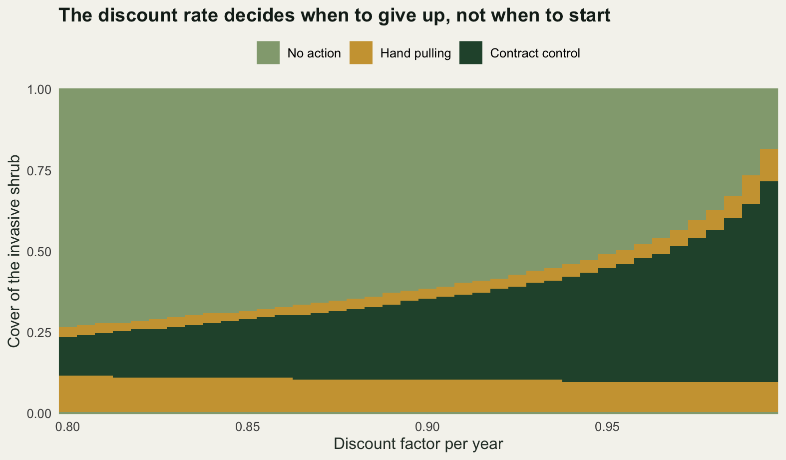
The lower boundary is almost immovable. Across the whole sweep the cover at which the contractor replaces the volunteers travels 0.0188, from 0.1156 at a discount factor of 0.80 to 0.0969 at 0.995. Whether you are patient or impatient, the contractor takes over at a cover close to a tenth of the reserve. The upper boundary travels 0.5500 over the same sweep, from 0.2656 to 0.8156. At a discount factor of 0.80, which is a discount rate of 25 per cent a year, the reserve is written off once the shrub passes a quarter of it. At 0.995 the rule is still sending crews out when four fifths of the reserve is gone.
Of the 161 states, 23 get a different action at a discount factor of 0.90 than at 0.95, and 46 do at 0.99. That is 14.3 and 28.6 per cent of the state space, which sounds like a mild sensitivity until the rules are priced against each other. Handing an impatient rule to a patient owner is the expensive direction: the 0.90 rule, judged by an objective with a discount factor of 0.99, costs 29.879 thousand pounds more than that objective’s own rule, which is 18.742 per cent. The reverse mistake, a patient rule judged by an impatient objective, costs 1.675 thousand or 3.175 per cent. Against the working objective of 0.95, the two wrong rules cost 1.558 and 2.149 per cent.
The asymmetry is worth carrying. Over-treating in the early years is a bounded error, because you are spending real money on a real problem slightly too early. Under-treating is not bounded, because the shrub goes on compounding while you fail to act, and by the time the mistake shows up the cover is past the point where any crew can hold the line. If the discount rate is uncertain, the cheaper direction to be wrong in is the patient one.
None of this is a calibration problem. Nobody can go out and measure the discount rate on a nature reserve. It encodes how a public body weighs a habitat now against the same habitat in thirty years, which is a question for the people who own the decision, and the honest way to present a rule like this one is with the discount factor written on the front of it rather than buried in the code.
Check 2: the state grid
The shrub’s cover is a continuous quantity and the model is a finite matrix, so somebody chose a grid. That choice is usually made on grounds of run time and reported nowhere. The check solves the same continuous problem on grids of 11, 41, 161 and 801 states, treats the 801 state answer as the truth, and evaluates each coarse rule against it by reading the coarse rule as a step function of cover and pricing it on the fine model.
grid_set <- c(11, 41, 161, 801)
to_ref <- function(pol, xs) pol[apply(abs(outer(x_ref, xs, "-")), 1, which.min)]
gres <- lapply(grid_set, function(n) {
  pl <- build_P(n); cc <- cost_of(n); ss <- solve_mdp(pl, cc); xs <- nodes_of(n)
  list(n = n, xs = xs, pol = ss$pol, own = ss$v, stay0 = pl[[1]][1, 1],
       true = eval_pol(p_ref, to_ref(ss$pol, xs), c_ref))
})
print(do.call(rbind, lapply(gres, function(z) data.frame(
  states = z$n,
  bottom_bin_edge = round(1 / (2 * (z$n - 1)), 5),
  prob_stay_at_zero = round(z$stay0, 4),
  claimed_cost_at_0.10 = round(approx(z$xs, z$own, 0.10)$y, 3),
  true_cost_at_0.10 = round(approx(x_ref, z$true, 0.10)$y, 3),
  extra_pct = round(100 * (mean(z$true[lo_ref]) - mean(ref$v[lo_ref])) /
                      mean(ref$v[lo_ref]), 3),
  extra_cost = round(mean(z$true[lo_ref]) - mean(ref$v[lo_ref]), 3)))),
  row.names = FALSE)
states bottom_bin_edge prob_stay_at_zero claimed_cost_at_0.10
11 0.05000 1.0000 22.500
41 0.01250 1.0000 22.500
161 0.00313 0.1617 33.952
801 0.00062 0.0000 31.516
true_cost_at_0.10 extra_pct extra_cost
87.036 79.340 54.763
39.794 10.937 7.549
32.186 0.860 0.593
31.516 0.000 0.000for (z in gres) cat("states", z$n, "boundaries at cover:",
paste(format(bounds_of(z$pol, z$xs), scientific = FALSE),
collapse = " "), "\n")states 11 boundaries at cover: 0.05 0.45 0.55
states 41 boundaries at cover: 0.0125 0.0875 0.4375 0.4875
states 161 boundaries at cover: 0.0031 0.0969 0.4469 0.4906
states 801 boundaries at cover: 0.0006 0.0981 0.4469 0.4894 library(grid)
band <- do.call(rbind, lapply(gres, function(z) {
hh <- 1 / (2 * (z$n - 1))
data.frame(states = z$n,
xmin = pmax(z$xs - hh, 0), xmax = pmin(z$xs + hh, 1),
action = factor(act_name[z$pol], levels = act_name))
}))
band$row <- match(band$states, grid_set)
lab_grid <- paste(grid_set, "states")
p_left <- ggplot(band) +
geom_rect(aes(xmin = xmin, xmax = xmax, ymin = row - 0.42, ymax = row + 0.42,
fill = action)) +
scale_fill_manual(values = act_col, name = NULL) +
scale_y_continuous(breaks = seq_along(grid_set), labels = lab_grid,
trans = "reverse") +
scale_x_continuous(expand = c(0, 0)) +
labs(x = "Cover of the invasive shrub", y = NULL,
title = "A coarse grid invents a permanent eradication") +
theme_te() +
theme(legend.position = "top", panel.grid.major.y = element_blank(),
plot.margin = margin(4, 14, 6, 6))
curve_df <- do.call(rbind, lapply(gres, function(z)
data.frame(cover = x_ref[lo_ref], cost = z$true[lo_ref],
grid = paste(z$n, "states"))))
curve_df$grid <- factor(curve_df$grid, levels = lab_grid)
p_right <- ggplot(curve_df, aes(cover, cost, colour = grid)) +
geom_line(linewidth = 0.9) +
scale_colour_manual(values = c(te_pal$clay, te_pal$gold, te_pal$green,
te_pal$forest), name = NULL) +
guides(colour = guide_legend(nrow = 1)) +
labs(x = "Cover at which the shrub is found",
y = "True cost, thousand pounds",
title = "The cost of a coarse grid lands at low cover") +
theme_te() +
theme(legend.position = "top", plot.margin = margin(4, 14, 6, 6))
grid.newpage()
pushViewport(viewport(layout = grid.layout(2, 1)))
print(p_left, vp = viewport(layout.pos.row = 1, layout.pos.col = 1))
print(p_right, vp = viewport(layout.pos.row = 2, layout.pos.col = 1))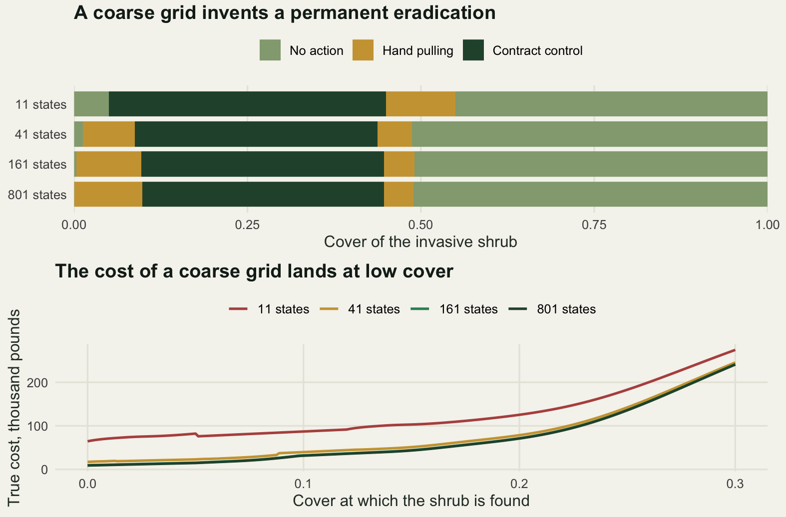
The 11 state rule costs 79.340 per cent more than the reference rule, which is 54.763 thousand pounds on an expected cost of 69.023. The 41 state rule costs 10.937 per cent, or 7.549 thousand. The 161 state rule costs 0.860 per cent. None of these grids is absurd. Eleven states is a sensible first pass, forty one is what most people would settle on, and a hundred and sixty one feels generous for a one dimensional problem.
The mechanism is in the third column of the table. On a grid of 11 states the lowest bin runs from zero to a cover of 0.05, and anything that lands in it is recorded as zero cover. From zero cover the seed rain puts next year’s median at 0.004, which is inside the same bin, so the probability of staying at zero once you arrive there is 1.0000. The model has an absorbing state. It believes that clearing the last few per cent of the shrub eradicates it permanently and for free, and it plans accordingly: clear hard, then stop. On the 41 state grid the bin edge is at 0.0125 and the same thing happens, again with probability 1.0000. Only at 161 states does the bottom bin start to leak, at 0.1617, and only at 801 does the model agree with the continuous process that the shrub always comes back.
That is why the coarse rules leave a visible band of untreated cover at the bottom of the upper panel: on the 11 state grid it runs up to a cover of 0.05, while on the 801 state grid it stops at 0.0006 and cannot be seen. The coarse model is not doing nothing because the shrub is gone. It is doing nothing because it thinks the shrub is gone. Followed on the real system, the rule clears the reserve, walks away, and comes back to the same problem a few years later, which is the cycle priced in the lower panel.
What the model says about itself is further out than what it recommends. At a cover of a tenth, the 11 state model reports an expected cost of 22.500 thousand pounds for its own rule. The true cost of that rule is 87.036. The 41 state model reports the same 22.500 against a true 39.794. Both are wrong in the reassuring direction, and neither model contains anything that would flag it. The 161 state model reports 33.952 against a true 32.186 and errs the other way, which is the first sign of a grid fine enough to be pessimistic rather than hopeful.
The boundaries tell the same story in cover units rather than grid indices, which is the only way to compare them. The 11 state rule switches at 0.05, 0.45 and 0.55. The 41 state rule switches at 0.0125, 0.0875, 0.4375 and 0.4875. The 161 state rule gives 0.0031, 0.0969, 0.4469 and 0.4906 against the reference 0.0006, 0.0981, 0.4469 and 0.4894. Reported as grid indices these look like different problems; reported as covers they are visibly converging, and the abandonment threshold is stable from 41 states upward. It is the low cover end that needs the resolution, because that is where the interesting question lives.
The general point is not that grids should be fine. It is that the grid is a modelling assumption about what outcomes exist, not a numerical setting. The bin width at the bottom of the state space decides whether eradication is a thing that can happen. Nothing in the output of a coarse solve says so, and refining until the value function stops moving is the cheapest check in this post.
Check 3: the transition matrix nobody estimated
The matrix was written from three stated numbers. Suppose instead there is a management record: a run of annual cover estimates with the action taken in each year, from a warden who used the contractor above a cover of 0.2, the volunteers between 0.05 and 0.2 and nothing below, with a one in four chance in any year of doing something else because of budget, weather or a contractor who did not turn up. Records of 20, 50 and 200 years are simulated from the true process, and three estimators are run on each of them.
The first fits the structural model with the seed rain assumed known, so two free parameters, by maximum likelihood on the log scale with the cover cap treated as a right censored observation. The second fits the same model with the seed rain free as well, so three parameters. The third refuses to assume a functional form and estimates the transition matrix by counting transitions on the working grid, with a weak uniform prior spread over every row, which is all that a row with no data has to go on. Each fitted matrix is solved and the resulting rule is priced on the true matrix.
hist_act <- function(x, u1, u2) {
  a <- if (x > 0.2) 3L else if (x > 0.05) 2L else 1L
  if (u1 < 0.25) a <- 1L + as.integer(u2 * 3)
  a
}
sim_series <- function(n_yr, x0 = 0.12) {
  x <- numeric(n_yr + 1); a <- integer(n_yr); x[1] <- x0
  for (k in 1:n_yr) {
    a[k] <- hist_act(x[k], runif(1), runif(1))
    x[k + 1] <- min(med_map(x[k], a[k]) * exp(log_sd * rnorm(1)), 1)
  }
  list(x = x, a = a)
}
neg_ll <- function(rr, sg, mm, yy, lxn, cen) {
  lz <- log(yy + rr * yy * (1 - yy) + mm * (1 - yy))
  ll <- numeric(length(lz))
  ll[!cen] <- dnorm(lxn[!cen], lz[!cen], sg, log = TRUE)
  ll[cen] <- pnorm(lz[cen] / sg, log.p = TRUE)
  -sum(ll)
}
prep <- function(sr) {
  x <- head(sr$x, -1); xn <- sr$x[-1]
  list(y = x - pmin(act_cap[sr$a], x), lxn = log(pmax(xn, 1e-12)),
       cen = xn >= 1 - 1e-12)
}
fit_two <- function(sr) {
  dd <- prep(sr)
  o <- optim(c(log(0.7), log(0.25)), function(p)
    neg_ll(exp(p[1]), exp(p[2]), seed_rain, dd$y, dd$lxn, dd$cen))
  c(r = exp(o$par[1]), s = exp(o$par[2]), m = seed_rain)
}
fit_three <- function(sr) {
  dd <- prep(sr)
  o <- optim(c(log(0.7), log(0.25), log(0.004)), function(p)
    neg_ll(exp(p[1]), exp(p[2]), exp(p[3]), dd$y, dd$lxn, dd$cen))
  c(r = exp(o$par[1]), s = exp(o$par[2]), m = exp(o$par[3]))
}
bin_of <- function(v, n) {
  xs <- nodes_of(n)
  as.integer(cut(v, c(-Inf, xs[-1] - 1 / (2 * (n - 1)), Inf), labels = FALSE))
}
emp_P <- function(sr, n) {
  ii <- bin_of(head(sr$x, -1), n); jj <- bin_of(sr$x[-1], n)
  lapply(seq_along(act_name), function(a) {
    mm <- matrix(1 / n, n, n)
    for (k in which(sr$a == a)) mm[ii[k], jj[k]] <- mm[ii[k], jj[k]] + 1
    mm / rowSums(mm)
  })
}
set.seed(20260724)
n_rep <- 120; len_set <- c(20, 50, 200); rows <- list()
for (n_yr in len_set) for (rp in 1:n_rep) {
  sr <- sim_series(n_yr)
  f2 <- fit_two(sr); f3 <- fit_three(sr)
  l2 <- loss_w(solve_mdp(build_P(n_w, f2["r"], f2["s"], f2["m"]), c_w)$pol)
  l3 <- loss_w(solve_mdp(build_P(n_w, f3["r"], f3["s"], f3["m"]), c_w)$pol)
  lc <- loss_w(solve_mdp(emp_P(sr, n_w), c_w)$pol)
  rows[[length(rows) + 1]] <- data.frame(years = n_yr,
    r2 = f2["r"], r3 = f3["r"], m3 = f3["m"],
    two = l2["extra_pct"], three = l3["extra_pct"], counts = lc["extra_pct"],
    counts_cost = lc["extra_cost"],
    cells = length(unique(paste(bin_of(head(sr$x, -1), n_w), sr$a))))
}
est <- do.call(rbind, rows)
c(replicates = n_rep, rows_in_the_matrix = n_w * length(act_name))
replicates rows_in_the_matrix
120 483 print(round(aggregate(cbind(r2, r3, m3, cells) ~ years, est, median), 4), row.names = FALSE) years r2 r3 m3 cells
20 0.7070 0.6313 0.0048 16
50 0.7173 0.6987 0.0041 29
200 0.7034 0.6943 0.0041 98print(round(aggregate(cbind(two, three, counts) ~ years, est, median), 3), row.names = FALSE) years two three counts
20 0.221 0.728 433.657
50 0.054 0.105 405.096
200 0.031 0.032 358.930print(round(aggregate(cbind(two, three, counts) ~ years, est,
function(z) quantile(z, 0.9)), 3), row.names = FALSE) years two three counts
20 2.104 229.797 445.421
50 0.607 1.454 446.383
200 0.249 0.830 463.412print(round(aggregate(counts_cost ~ years, est, median), 3), row.names = FALSE) years counts_cost
20 297.327
50 277.745
200 246.092e20 <- est[est$years == 20, ]
round(c(share_three_above_5pct_at_20y = mean(e20$three > 5),
share_two_above_5pct_at_20y = mean(e20$two > 5),
spearman_seed_rain_vs_loss = cor(e20$m3, e20$three, method = "spearman"),
seed_rain_q90_at_20y = quantile(e20$m3, 0.9)), 4)share_three_above_5pct_at_20y share_two_above_5pct_at_20y
0.1833 0.0333
spearman_seed_rain_vs_loss seed_rain_q90_at_20y.90%
0.5169 0.0737 round(loss_w(solve_mdp(build_P(n_w, mm = 0.07), c_w)$pol), 3)extra_cost extra_pct
52.623 76.751 est_lab <- c("Two parameters", "Three parameters", "Transition counts")
long <- rbind(
data.frame(years = est$years, loss = est$two, estimator = est_lab[1]),
data.frame(years = est$years, loss = est$three, estimator = est_lab[2]),
data.frame(years = est$years, loss = est$counts, estimator = est_lab[3]))
long$estimator <- factor(long$estimator, levels = est_lab)
long$years <- factor(long$years, levels = len_set, labels = paste(len_set, "years"))
long$loss <- pmax(long$loss, 0.01)
ggplot(long, aes(years, loss, fill = estimator)) +
geom_boxplot(colour = te_pal$ink, linewidth = 0.35, outlier.size = 0.7,
alpha = 0.75) +
scale_fill_manual(values = c(te_pal$forest, te_pal$gold, te_pal$clay), name = NULL) +
scale_y_log10(breaks = c(0.01, 0.1, 1, 10, 100, 1000),
labels = c("0.01", "0.1", "1", "10", "100", "1000")) +
labs(x = "Length of the management record", y = "Extra cost, per cent",
title = "One extra parameter is what makes short records dangerous") +
theme_te() +
theme(legend.position = "top")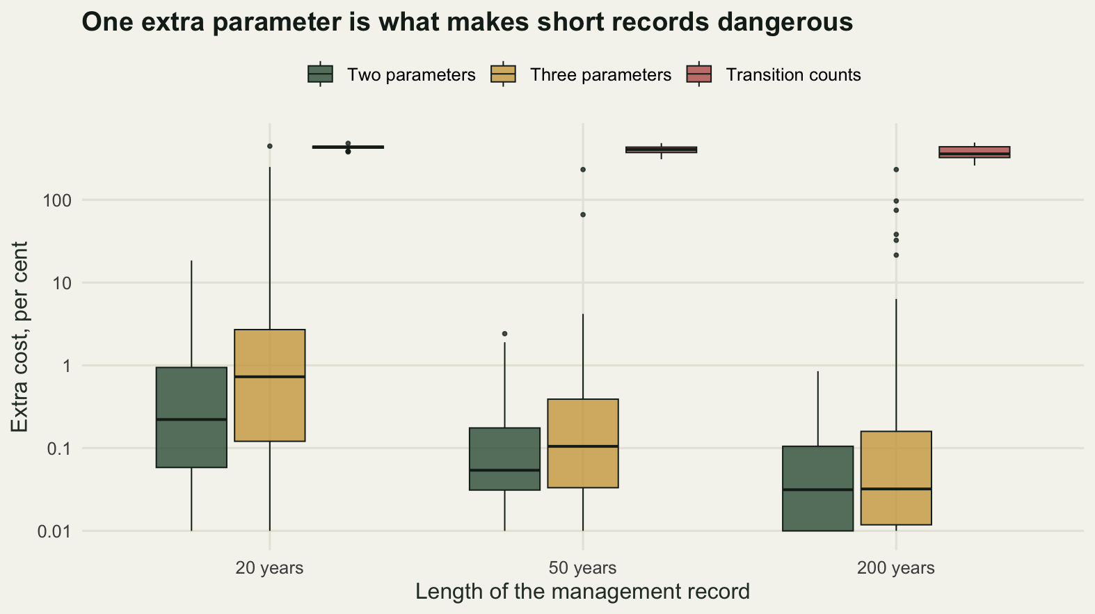
The two parameter fit is almost harmless. Its median extra cost is 0.221 per cent from a 20 year record, 0.054 per cent from 50 years and 0.031 per cent from 200, and its median spread rate estimates are 0.7070, 0.7173 and 0.7034 against a true 0.7. For the median record, twenty annual cover estimates are enough to recover a rule that is within half a per cent of the right one, though the worst tenth of records run several times higher. That is not what the framing of this check expected, and it is the result.
Adding one parameter changes the picture. With the seed rain free as well, the median loss from a 20 year record is 0.728 per cent, which still looks fine, but on this run the ninetieth percentile is 229.797 per cent against 2.104 for the two parameter fit, and 0.1833 of the 20 year records produce a rule that costs more than five per cent extra. The tail is the whole story: most records are fine and the ones that are not cost many times the median. By 50 years the ninetieth percentile has fallen to 1.454 per cent and by 200 years to 0.830.
The reason is exactly the mechanism of check 2, arriving this time through the data rather than through the grid. The seed rain is a small number that only matters at low cover, and the record was made at covers where it is a rounding error, so it is barely identified. Its ninetieth percentile estimate from 20 years is 0.0737, against a true 0.004, and its rank correlation with the loss is 0.5169. A model that believes in a seed rain of 0.07 believes the reserve is under constant re-invasion from outside, gives up on the low cover states, and costs 76.751 per cent extra when its rule is priced on the truth. Check 2 found a model that was too optimistic about eradication because of a bin edge. Check 3 finds one that is too pessimistic about it because of a parameter the data never saw.
The transition count estimator is in a different category. Its median loss is 433.657 per cent from 20 years, 405.096 from 50 and 358.930 from 200, which in money is between 246.092 and 297.327 thousand pounds of extra expected cost. The trend with data is real and useless. The reason is in the count above the table: the matrix has 483 rows, being 161 states by three actions, and the median number of rows with any data at all is 16 from a 20 year record, 29 from 50 years and 98 from 200. Two centuries of annual monitoring fills a fifth of the object. Coarsening the grid so that the counting becomes feasible is not an escape either, since check 2 has already priced an 11 state grid at 79.340 per cent.
So the transition matrix in a sequential decision model is not data. It is a model with two or three parameters in it, wearing a matrix as a costume, and the honest way to report one is to give the parameters and their sources rather than the matrix. The check that matters is not whether the matrix was estimated well. It is which parameters the record could actually see, and whether the ones it could not see are the ones the rule turns on.
Check 4: the end of the horizon
Management plans have end dates. A five year plan, a ten year scheme, a twenty five year vision: each of those is a finite horizon problem, and the finite horizon problem is solved by backward induction from a terminal condition rather than by iterating to a fixed point. The usual terminal condition is nothing, meaning the world is assumed to end with the plan. The check runs backward induction over 40 years and compares each step with the stationary rule.
n_hz <- 40
v_t <- rep(0, n_w); pol_t <- matrix(0L, n_w, n_hz); v_hz <- matrix(0, n_w, n_hz)
for (k in 1:n_hz) {
  qq <- sapply(seq_along(act_name), function(a) c_w[, a] + dfac * (p_w[[a]] %*% v_t))
  pol_t[, k] <- max.col(-qq, ties.method = "first")
  v_t <- qq[cbind(seq_len(n_w), pol_t[, k])]
  v_hz[, k] <- v_t
}
diff_k <- apply(pol_t, 2, function(p) sum(p != base$pol))
gu_t <- apply(pol_t, 2, function(p) {
  k <- which(p != 1); if (!length(k)) 0 else (x_w[max(k)] + x_w[max(k) + 1]) / 2 })
kshow <- c(1, 2, 5, 10, 20, 30, 40)
print(data.frame(years_left = kshow, states_differing = diff_k[kshow],
                 abandon_above = round(gu_t[kshow], 4)), row.names = FALSE)
years_left states_differing abandon_above
1 78 0.0000
2 78 0.0000
5 54 0.3094
10 30 0.3469
20 17 0.4156
30 12 0.4531
40 7 0.4656round(c(stationary_abandon_above = (x_w[max(which(base$pol != 1))] +
x_w[max(which(base$pol != 1)) + 1]) / 2,
horizon_40_cost = mean(v_hz[lo_w, n_hz]),
infinite_cost = mean(base$v[lo_w]),
understated_pct = 100 * (mean(base$v[lo_w]) - mean(v_hz[lo_w, n_hz])) /
mean(base$v[lo_w])), 3)stationary_abandon_above horizon_40_cost infinite_cost
0.491 65.129 68.563
understated_pct
5.008 fin_val <- function(pol_fixed, tp) {
vv <- rep(0, n_w)
for (k in 1:tp) {
pp <- matrix(0, n_w, n_w)
for (a in seq_along(act_name)) {
ii <- which(pol_fixed == a)
if (length(ii)) pp[ii, ] <- p_w[[a]][ii, , drop = FALSE]
}
vv <- c_w[cbind(seq_len(n_w), pol_fixed)] + dfac * (pp %*% vv)
}
as.vector(vv)
}
print(do.call(rbind, lapply(c(5, 10, 20, 40), function(tp) {
vs <- fin_val(base$pol, tp)
data.frame(plan_years = tp,
plan_used_for_ever_pct = round(loss_w(pol_t[, tp])["extra_pct"], 3),
stationary_used_for_plan_pct = round(100 * (mean(vs[lo_w]) -
mean(v_hz[lo_w, tp])) / mean(v_hz[lo_w, tp]), 3))
})), row.names = FALSE) plan_years plan_used_for_ever_pct stationary_used_for_plan_pct
5 148.896 37.305
10 5.983 4.809
20 0.517 1.140
40 0.033 0.232v_t2 <- base$v; n_diff2 <- 0L
for (k in 1:n_hz) {
qq <- sapply(seq_along(act_name), function(a) c_w[, a] + dfac * (p_w[[a]] %*% v_t2))
pk <- max.col(-qq, ties.method = "first")
n_diff2 <- n_diff2 + sum(pk != base$pol)
v_t2 <- qq[cbind(seq_len(n_w), pk)]
}
c(states_differing_with_stationary_terminal_value = n_diff2,
state_steps_checked = n_w * n_hz)states_differing_with_stationary_terminal_value
0
state_steps_checked
6440 hz_map <- data.frame(
years_left = rep(seq_len(n_hz), each = n_w),
cover = rep(x_w, n_hz),
action = factor(act_name[as.vector(pol_t)], levels = act_name))
st_bounds <- bounds_of(base$pol, x_w)
ggplot(hz_map, aes(years_left, cover, fill = action)) +
geom_raster() +
geom_hline(yintercept = st_bounds[2:4], colour = te_pal$ink,
linetype = "22", linewidth = 0.5) +
scale_fill_manual(values = act_col, name = NULL) +
scale_x_continuous(expand = c(0, 0)) +
scale_y_continuous(expand = c(0, 0)) +
labs(x = "Years remaining in the plan", y = "Cover of the invasive shrub",
title = "A finite horizon changes the rule decades before the end",
subtitle = paste("Dashed lines: the three action boundaries of the same rule",
"solved with no end to the horizon")) +
theme_te() +
theme(legend.position = "top",
plot.subtitle = element_text(size = 9.5, colour = "#2c3a31"))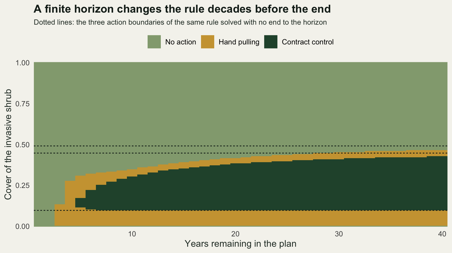
With one or two years left, the rule is to do nothing anywhere. All 78 states that the stationary rule would treat are left alone, because a crew sent out in the final year buys a reduction in cover that nobody will be around to enjoy. With five years left the abandonment threshold is 0.3094 and 54 states still disagree with the stationary rule. With ten years left it is 0.3469 and 30 states. With twenty it is 0.4156 and 17 states, with thirty 0.4531 and 12, and with forty 0.4656 and 7. The stationary threshold is 0.491, and the finite horizon solution has not reached it after forty years.
That is the honest correction to the way this check is usually described. The end of the horizon does not distort the last few steps. At a discount factor of 0.95 it distorts everything, decaying geometrically, and forty years back the rule is still visibly different and the value function still understates the infinite horizon cost by 5.008 per cent, 65.129 thousand pounds against the working grid’s 68.563 (the 801 state reference figure quoted earlier is 69.023). A plan long enough that its ending does not matter would have to be several times longer than any management plan ever written.
The prices of the two possible mistakes are not equal. Taking the first year of a five year plan and using it as standing policy costs 148.896 per cent extra, which is the outcome of writing off a reserve that a longer view would still be defending. Ten years costs 5.983 per cent, twenty 0.517 and forty 0.033. In the other direction, running the stationary rule inside a genuine five year problem costs 37.305 per cent, ten years 4.809, twenty 1.140 and forty 0.232. Both mistakes are expensive at five years and both are cheap at twenty, but the five year comparison is lopsided: the short plan used for ever costs about four times what the long rule used briefly does, and it fails in the direction of doing too little.
The fix costs one line. Backward induction with the stationary value function as the terminal condition, rather than zero, reproduces the stationary rule exactly: across 6440 state and step combinations, 0 differ. The terminal condition is a statement about what the reserve is worth on the day the plan expires, and setting it to zero says the reserve is worth nothing then. Nobody believes that, and it is written into most finite horizon code by default.
What the four checks cannot see
All four checks assume the state is known when the action is chosen. The rule is a function of cover, and it has been fed the true cover every time. Real management reads the cover off a survey.
The last block leaves the grid behind entirely and simulates the continuous process forward from starting covers drawn from the same discovery set, applying the 801 state rule to whatever the survey reported. Three versions are run on identical random draws: a perfect survey, a survey with a lognormal error a little larger than one year of the process noise, and the same noisy survey with a three in ten chance of missing an infestation below five per cent cover altogether.
set.seed(20260724)
n_sim <- 4000; n_yr_sim <- 120
start_pool <- x_ref[lo_ref]
pol_fun <- function(xo) ref$pol[pmax(1L, pmin(n_ref, round(xo * (n_ref - 1)) + 1L))]
run_sim <- function(obs_sd, miss_p, x0) {
  x <- x0; tot <- rep(0, n_sim)
  for (k in 1:n_yr_sim) {
    xo <- if (obs_sd > 0) pmin(x * exp(obs_sd * rnorm(n_sim)), 1) else x
    if (miss_p > 0) xo[x < 0.05 & runif(n_sim) < miss_p] <- 0
    a <- pol_fun(xo)
    tot <- tot + dfac^(k - 1) * stage_cost(x, a)
    x <- pmin(med_map(x, a) * exp(log_sd * rnorm(n_sim)), 1)
  }
  mean(tot)
}
x0_pool <- sample(start_pool, n_sim, replace = TRUE)
set.seed(20260724); s_perfect <- run_sim(0, 0, x0_pool)
set.seed(20260724); s_noisy   <- run_sim(0.30, 0, x0_pool)
set.seed(20260724); s_missed  <- run_sim(0.30, 0.30, x0_pool)
c(replicates = n_sim, years_simulated = n_yr_sim)
replicates years_simulated
4000 120 round(c(observation_log_sd = 0.30, non_detection_below_0.05 = 0.30,
analytic_cost = mean(ref$v[lo_ref]), simulated_cost = s_perfect,
calibration_gap_pct = 100 * (s_perfect - mean(ref$v[lo_ref])) /
mean(ref$v[lo_ref])), 3) observation_log_sd non_detection_below_0.05 analytic_cost
0.300 0.300 69.023
simulated_cost calibration_gap_pct
68.896 -0.184 round(c(perfect = s_perfect, noisy = s_noisy, noisy_and_missed = s_missed,
noisy_pct = 100 * (s_noisy - s_perfect) / s_perfect,
missed_pct = 100 * (s_missed - s_perfect) / s_perfect), 3) perfect noisy noisy_and_missed noisy_pct
68.896 76.604 81.208 11.187
missed_pct
17.870 The perfect survey run doubles as the last calibration in the post, and it is the one that justifies everything above it. Simulating the continuous process directly, with no grid anywhere in the loop except in the lookup of the action, gives an expected discounted cost of 68.896 thousand pounds against the 69.023 that the 801 state model computed by linear algebra. The simulation and the linear algebra differ by 0.184 per cent, which is the truncation at 120 years plus Monte Carlo error over 4000 replicates. The discretised model is a fair account of the continuous one.
A survey with a lognormal error of 0.30 on the log scale costs 11.187 per cent, taking the expected cost to 76.604 thousand. Adding a three in ten chance of missing a low cover infestation takes it to 81.208, or 17.870 per cent above perfect information. That is comparable to handing a patient owner an impatient rule, which cost 18.742 per cent in check 1, and rather more than a 41 state grid costs at 10.937 per cent. It is invisible to all four checks, because all four ask what the rule should be given the state and none asks what happens when the state is read wrong.
The proper treatment is a partially observed model, where the state is a probability distribution over covers rather than a cover, and the rule is a function of that distribution. Those are expensive to solve and rare in practice. The cheap alternative is the one run here: keep the rule you have, simulate it forward through the observation process you actually have, and price the difference. It takes a few lines, it needs no new theory, and it is the only one of the five numbers in this post that a monitoring budget can act on.
There is a second thing none of the checks can see, and it cannot be measured from inside the model at all. Every check above assumes the shrub spreads logistically with lognormal noise, and the truth against which everything was scored was built from that same assumption. A dispersal kernel with a long tail, a seed bank that carries the infestation through a year of apparently clean ground, or a neighbour who changes their management, would each break the state description rather than the numbers in it. Checks 1 to 4 measure how much of the rule depends on choices made after the state variable was chosen. The choice of the state variable itself is upstream of all of them.
Where to go next
The three posts this one is checking build the machinery. Markov decision processes for management sets out the state, the action set, the transition matrix and the Bellman equation, and shows why the output of value iteration is a stationary rule. Stochastic dynamic programming for harvest derives an optimal harvest rule and measures how far it sits from constant escapement once uncertainty and a concave utility are switched on. When to stop monitoring is the optimal stopping version of the same idea, and it is the natural next step after the observation error result above, since it prices the information a survey buys against what the survey costs and what the delay costs.
If you take one habit from this post, make it the grid refinement in check 2. It costs one extra solve, and it is the only one of the four failures that the model reports as good news: a coarse solve hands back a lower expected cost and no warning at all.
References
Puterman ML 1994 Markov Decision Processes: Discrete Stochastic Dynamic Programming. Wiley, ISBN 978-0-471-61977-2
Marescot L, Chapron G, Chades I, Fackler PL, Duchamp C, Marboutin E, Gimenez O 2013 Methods in Ecology and Evolution 4(9):872-884 (10.1111/2041-210X.12082)
Chades I, Chapron G, Cros MJ, Garcia F, Sabbadin R 2014 Ecography 37(9):916-920 (10.1111/ecog.00888)
Clark CW, Mangel M 2000 Dynamic State Variable Models in Ecology: Methods and Applications. Oxford University Press, ISBN 978-0-19-512267-1
Sutton RS, Barto AG 2018 Reinforcement Learning: An Introduction. Second edition. MIT Press, ISBN 978-0-262-03924-6
Weitzman ML 2001 American Economic Review 91(1):260-271 (10.1257/aer.91.1.260)