library(ggplot2)

te_pal <- list(forest = "#275139", green = "#2f8f63", sage = "#93a87f",
               clay = "#b5534e", gold = "#cda23f", line = "#dad9ca",
               ink = "#16241d", paper = "#f5f4ee")

theme_te <- function() {
  theme_minimal(base_size = 12) +
    theme(panel.grid.minor = element_blank(),
          panel.grid.major = element_line(colour = "#e7e6dc"),
          plot.background = element_rect(fill = "#f5f4ee", colour = NA),
          panel.background = element_rect(fill = "#f5f4ee", colour = NA),
          plot.title = element_text(face = "bold", colour = te_pal$ink),
          axis.title = element_text(colour = "#2c3a31"))
}Markov decision processes for management
R
conservation
decision analysis
ecology tutorial
ggplot2
Build a Markov decision process for an invasive plant in R, solve it by value iteration, and measure what a one year view of the same problem costs a reserve.
Himalayan balsam turns up in one of the ten compartments a warden walks each summer. She has three options this winter, and the same three every winter after it: leave it, send two people with knapsack sprayers into the compartments that have it, or put a contractor across the whole site. Whichever she picks, next summer’s map is not this summer’s map, and what she should do next winter depends on the map she gets.
That last sentence is what makes this a different kind of problem from a consequence table. There is no single decision to rank options for. There is a state that moves, an action that moves it, and a question that comes back every year, so the thing worth computing is not an action but a rule: an action for every state the site could be in. This tutorial builds that rule for the balsam problem and measures four things about it. Whether the arithmetic is right, checked by solving the same quantity a second way with linear algebra. What the one year view of the problem costs. Where the discount factor changes what the rule says. And how much of the rule survives a transition matrix that is 10 per cent wrong.
The blog already has three decision analysis tutorials and this one sits outside all of them. Structured decision making in R ranks a fixed set of options against a fixed set of consequences, once. The expected value of information prices the uncertainty in that one shot decision before it is taken. Adaptive management and learning repeats a decision while the manager’s belief about a fixed world improves. Here the world itself moves: the plant spreads between compartments whether or not anyone is watching, and this winter’s spraying is the reason next winter’s map looks the way it does.
The site, the actions and the money
The reserve is cut into ten compartments and the state of the site is the number of them holding balsam, so there are eleven states from a clean site to a fully invaded one. The warden observes that number every summer and acts on it every winter. Doing nothing costs nothing. Spot treatment sends a crew to the invaded compartments, so it costs a fixed mobilisation charge plus a charge per invaded compartment, and it clears about six in ten of the treated compartments. Whole site control puts a contractor across all ten compartments whether they hold balsam or not, so it costs the same whatever the state, and it clears about nine in ten.
Damage is what the balsam does to the reserve, in the same money units, and it rises faster than the area it occupies because a compartment surrounded by invaded compartments is worth less than an isolated one. The convention on timing matters and is stated once here: the treatment cost is paid in the winter, the damage is charged on the cover the following summer, so the reward for taking an action in a state is minus the treatment cost minus the expected damage after the state has moved.
n_cell  <- 10L
states  <- 0:n_cell
n_s     <- length(states)
n_a     <- 3L
act_lab <- c("do nothing", "spot treatment", "whole site control")

kill  <- c(0, 0.60, 0.90)
mob   <- 1
per   <- 2.2
blank <- 28
d_max <- 60
d_pow <- 1.5
disc  <- 0.95

ext   <- 0.06
a_col <- 0.12
rain  <- 0.002

damage   <- d_max * (states / n_cell)^d_pow
cost_mat <- cbind(rep(0, n_s), mob + per * states, rep(blank, n_s))
colnames(cost_mat) <- act_lab

round(c(compartments = n_cell, states = n_s, actions = n_a,
        clearance_spot = kill[2], clearance_whole = kill[3],
        mobilisation = mob, cost_per_compartment = per, whole_site_cost = blank,
        damage_at_full_cover = d_max, damage_exponent = d_pow,
        discount_factor = disc, local_extinction = ext,
        neighbour_colonisation = a_col, arrival_from_outside = rain), 4)
compartments states actions
10.000 11.000 3.000
clearance_spot clearance_whole mobilisation
0.600 0.900 1.000
cost_per_compartment whole_site_cost damage_at_full_cover
2.200 28.000 60.000
damage_exponent discount_factor local_extinction
1.500 0.950 0.060
neighbour_colonisation arrival_from_outside
0.120 0.002 round(c(annual_discount_rate_percent = 100 * (1 / disc - 1)), 3)annual_discount_rate_percent
5.263 print(round(cbind(cells = states, damage = damage, cost_mat), 3)) cells damage do nothing spot treatment whole site control
[1,] 0 0.000 0 1.0 28
[2,] 1 1.897 0 3.2 28
[3,] 2 5.367 0 5.4 28
[4,] 3 9.859 0 7.6 28
[5,] 4 15.179 0 9.8 28
[6,] 5 21.213 0 12.0 28
[7,] 6 27.885 0 14.2 28
[8,] 7 35.140 0 16.4 28
[9,] 8 42.933 0 18.6 28
[10,] 9 51.229 0 20.8 28
[11,] 10 60.000 0 23.0 28Damage runs from 0 on a clean site to 60 thousand a year at full cover, and it is 9.859 at three invaded compartments against 21.213 at five, so the third compartment to be invaded costs the reserve less than the fifth. Spot treatment on three compartments costs 7.6 thousand; the contractor costs 28 thousand whether there are three invaded compartments or ten. That crossover in the cost structure is the reason the rule below has any shape at all.
The transition matrix comes from a patch occupancy model rather than from anyone’s judgement about what the numbers should be. Each invaded compartment survives the winter treatment with probability one minus the clearance rate, and then dies out on its own with probability 0.06, which leaves a binomial number of survivors. Each empty compartment is then colonised over the summer, with a probability that rises with the number of survivors nearby and has a small floor of 0.002 for arrivals from outside the reserve. Convolving the two binomials gives one row of the matrix for each state and action.
colonise <- function(m) 1 - (1 - rain) * exp(-a_col * m)

trans_row <- function(i, a) {
  surv <- (1 - kill[a]) * (1 - ext)
  p_surv <- dbinom(0:i, i, surv)
  out <- numeric(n_s)
  for (m in 0:i) {
    free <- n_cell - m
    out[(m:n_cell) + 1] <- out[(m:n_cell) + 1] +
      p_surv[m + 1] * dbinom(0:free, free, colonise(m))
  }
  out
}

trans <- array(0, c(n_s, n_a, n_s))
for (i in states) for (a in seq_len(n_a)) trans[i + 1, a, ] <- trans_row(i, a)
signif(c(largest_row_sum_error = max(abs(apply(trans, c(1, 2), sum) - 1))), 3)
largest_row_sum_error
2.22e-16 nxt <- sapply(seq_len(n_a), function(a) trans[, a, ] %*% states)
colnames(nxt) <- act_lab
print(round(cbind(cells = states, nxt), 3)) cells do nothing spot treatment whole site control
[1,] 0 0.020 0.020 0.020
[2,] 1 1.913 0.777 0.209
[3,] 2 3.516 1.488 0.396
[4,] 3 4.870 2.155 0.579
[5,] 4 6.009 2.781 0.760
[6,] 5 6.964 3.367 0.938
[7,] 6 7.761 3.917 1.113
[8,] 7 8.423 4.432 1.286
[9,] 8 8.970 4.915 1.455
[10,] 9 9.418 5.366 1.623
[11,] 10 9.782 5.788 1.787stat_dist <- function(m_mat) {
v <- rep(1 / n_s, n_s)
for (k in 1:5000) v <- as.vector(v %*% m_mat)
v
}
hit_time <- function(m_mat, target) {
keep <- which(states < target)
solve(diag(length(keep)) - m_mat[keep, keep], rep(1, length(keep)))
}
round(c(untreated_equilibrium_cells = sum(stat_dist(trans[, 1, ]) * states),
years_from_one_cell_to_five = hit_time(trans[, 1, ], 5)[2],
years_from_two_cells_to_five = hit_time(trans[, 1, ], 5)[3]), 3) untreated_equilibrium_cells years_from_one_cell_to_five
9.647 8.562
years_from_two_cells_to_five
2.813 The rows sum to one to within 2.22e-16, which is the only thing about a hand built transition matrix that can be checked without leaving the desk. Left alone, three invaded compartments become 4.87 by the next summer; spot treatment turns them into 2.155 and the contractor into 0.579. An untreated invasion settles at 9.647 of the ten compartments, so this is a plant that takes the site if nobody stops it.
The two waiting times are worth reading together. From two invaded compartments the site reaches five in 2.813 years on average. From one it takes 8.562 years, which is not because the spread is slower but because a single occupied compartment has a 6 per cent chance of dying out on its own, after which the site waits for the next arrival from outside, and those long waits sit inside the average.
Everything in this post now rests on that matrix, and it is worth saying plainly what it is. It is assumed, not estimated. No balsam was counted to produce it. The clearance rates, the extinction probability and the colonisation curve are a model of how this kind of plant behaves, written down so that it can be argued with, and the last section of this post measures what happens when it is wrong.
rewards <- function(tr) {
  out <- matrix(0, n_s, n_a, dimnames = list(states, act_lab))
  for (a in seq_len(n_a)) out[, a] <- -(cost_mat[, a] + tr[, a, ] %*% damage)
  out
}
rew <- rewards(trans)
print(round(-rew, 3))
do nothing spot treatment whole site control
0 0.038 1.038 28.038
1 5.592 5.460 28.594
2 13.133 10.199 29.169
3 20.978 15.149 29.762
4 28.465 20.227 30.372
5 35.300 25.372 30.997
6 41.367 30.536 31.636
7 46.641 35.683 32.288
8 51.150 40.785 32.950
9 54.948 45.820 33.623
10 58.103 50.775 34.304Read that table as this year’s bill under each action: the treatment cost plus the damage expected next summer. At three invaded compartments the three bills are 20.978, 15.149 and 29.762 thousand, so the cheapest thing to do this year is spot treatment. Hold that number.
The Bellman equation and two ways to solve it
The value of a state under a rule is this year’s reward plus the discounted value of wherever the site ends up, averaged over the transition. Written for the best rule rather than a given one, that is the Bellman equation, and its solution is a fixed point: the value of a state is the best over the three actions of the immediate reward plus the discount factor times the expected value of the next state. Value iteration turns that equation into an assignment and applies it until it stops changing.
A discount factor of 0.95 is an annual discount rate of 5.263 per cent, which is inside the range public bodies use. It is not a property of the balsam. Nothing in the ecology of the plant says how a reserve should weigh a cost this year against the same cost twenty years from now.
value_iter <- function(tr, rw, dsc, n_it) {
  v <- numeric(n_s)
  q <- matrix(0, n_s, n_a)
  sup <- numeric(n_it)
  spn <- numeric(n_it)
  for (k in seq_len(n_it)) {
    for (a in seq_len(n_a)) q[, a] <- rw[, a] + dsc * (tr[, a, ] %*% v)
    v_new <- apply(q, 1, max)
    step <- v_new - v
    sup[k] <- max(abs(step))
    spn[k] <- diff(range(step))
    v <- v_new
  }
  list(v = v, policy = apply(q, 1, which.max), sup = sup, span = spn)
}

policy_value <- function(tr, rw, dsc, pol) {
  p_pol <- t(sapply(seq_len(n_s), function(i) tr[i, pol[i], ]))
  solve(diag(n_s) - dsc * p_pol, rw[cbind(seq_len(n_s), pol)])
}

policy_iter <- function(tr, rw, dsc) {
  pol <- rep(1L, n_s)
  q <- matrix(0, n_s, n_a)
  for (k in 1:60) {
    v <- policy_value(tr, rw, dsc, pol)
    for (a in seq_len(n_a)) q[, a] <- rw[, a] + dsc * (tr[, a, ] %*% v)
    pol_new <- apply(q, 1, which.max)
    if (identical(pol_new, pol)) break
    pol <- pol_new
  }
  list(v = policy_value(tr, rw, dsc, pol), policy = pol, sweeps = k)
}

n_it <- 700
vi <- value_iter(trans, rew, disc, n_it)
pi_sol <- policy_iter(trans, rew, disc)
v_exact <- policy_value(trans, rew, disc, vi$policy)

c(iterations = n_it, policy_iteration_sweeps = pi_sol$sweeps,
  same_policy = identical(vi$policy, pi_sol$policy))
iterations policy_iteration_sweeps same_policy
700 3 1 signif(c(value_iteration_against_linear_solve = max(abs(vi$v - v_exact)),
value_iteration_against_policy_iteration = max(abs(vi$v - pi_sol$v))), 3) value_iteration_against_linear_solve
2.13e-14
value_iteration_against_policy_iteration
2.13e-14 Two independent routes to the same eleven numbers. Value iteration applies the Bellman operator 700 times from a standing start. Policy evaluation solves the linear system \((I - \gamma P_\pi) V_\pi = r_\pi\) directly for the rule value iteration produced, which involves no iteration at all and only agrees if the rule really is optimal. The largest disagreement between them is 2.13e-14, which is the floor for double precision arithmetic on numbers of this size. Policy iteration, a third route, reaches the same rule in 3 sweeps.
The way the error falls is more interesting than the fact that it falls.
floor_at <- 1e-12
sup_ok <- which(vi$sup > floor_at)
sup_ok <- sup_ok[sup_ok > 10]
spn_ok <- which(vi$span > floor_at)
spn_ok <- spn_ok[spn_ok > 5]
rate_sup <- median(vi$sup[sup_ok[-1]] / vi$sup[head(sup_ok, -1)])
rate_spn <- median(vi$span[spn_ok[-1]] / vi$span[head(spn_ok, -1)])

p_opt <- t(sapply(seq_len(n_s), function(i) trans[i, vi$policy[i], ]))
eig <- sort(Mod(eigen(p_opt, only.values = TRUE)$values), decreasing = TRUE)

round(c(measured_sup_norm_rate = rate_sup, discount_factor = disc,
        measured_span_rate = rate_spn, second_eigenvalue = eig[2],
        discount_times_second_eigenvalue = disc * eig[2]), 6)
measured_sup_norm_rate discount_factor
0.950000 0.950000
measured_span_rate second_eigenvalue
0.400534 0.421615
discount_times_second_eigenvalue
0.400534 c(sweeps_for_sup_norm_below_1e_9 = min(which(vi$sup < 1e-9)),
sweeps_for_span_below_1e_9 = min(which(vi$span < 1e-9)))sweeps_for_sup_norm_below_1e_9 sweeps_for_span_below_1e_9
385 29 The largest change in any state shrinks by a factor of 0.95 per sweep, which is the discount factor exactly, and that is the textbook contraction. The span of the change, meaning the gap between the state that moves most and the state that moves least, shrinks by 0.400534 per sweep instead. That number is not a coincidence and it is not an artefact: the second largest eigenvalue modulus of the transition matrix under the optimal rule is 0.421615, and 0.95 times 0.421615 is 0.400534 to six decimal places. The sup norm needs 385 sweeps to fall below one part in a billion and the span needs 29.
The practical consequence is that the differences between states settle long before the values do. Adding a constant to every state changes no comparison between actions, so the rule is fixed once the span has collapsed, and everything after that only pins down the absolute level. That is why span based stopping rules exist, and why a solver that has clearly not converged can still be returning the right rule.
kk <- seq_len(n_it)
cvg <- data.frame(
  iter = rep(kk, 2),
  y = log10(c(vi$sup, vi$span)),
  what = rep(c("largest change in any state", "span of the change across states"),
             each = n_it))
cvg <- cvg[is.finite(cvg$y) & cvg$y > -12, ]
gline <- data.frame(
  iter = rep(kk, 2),
  y = c(log10(vi$sup[12]) + (kk - 12) * log10(disc),
        log10(vi$span[7]) + (kk - 7) * log10(rate_spn)),
  what = rep(c("largest change in any state", "span of the change across states"),
             each = n_it))
gline <- gline[gline$y > -12 & gline$iter >= rep(c(12, 7), each = n_it), ]

ggplot(cvg, aes(iter, y, colour = what)) +
  geom_line(data = gline, aes(group = what), linewidth = 3, colour = "#c8c7b6") +
  geom_line(linewidth = 0.8) +
  scale_colour_manual(values = c(te_pal$clay, te_pal$forest), name = NULL) +
  scale_y_continuous(breaks = seq(-12, 3, by = 3),
                     labels = c("0.000000000001", "0.000000001", "0.000001",
                                "0.001", "1", "1000")) +
  labs(x = "Value iteration sweep", y = "Change in the value function",
       title = "The rule settles long before the values do") +
  theme_te() +
  theme(legend.position = "top")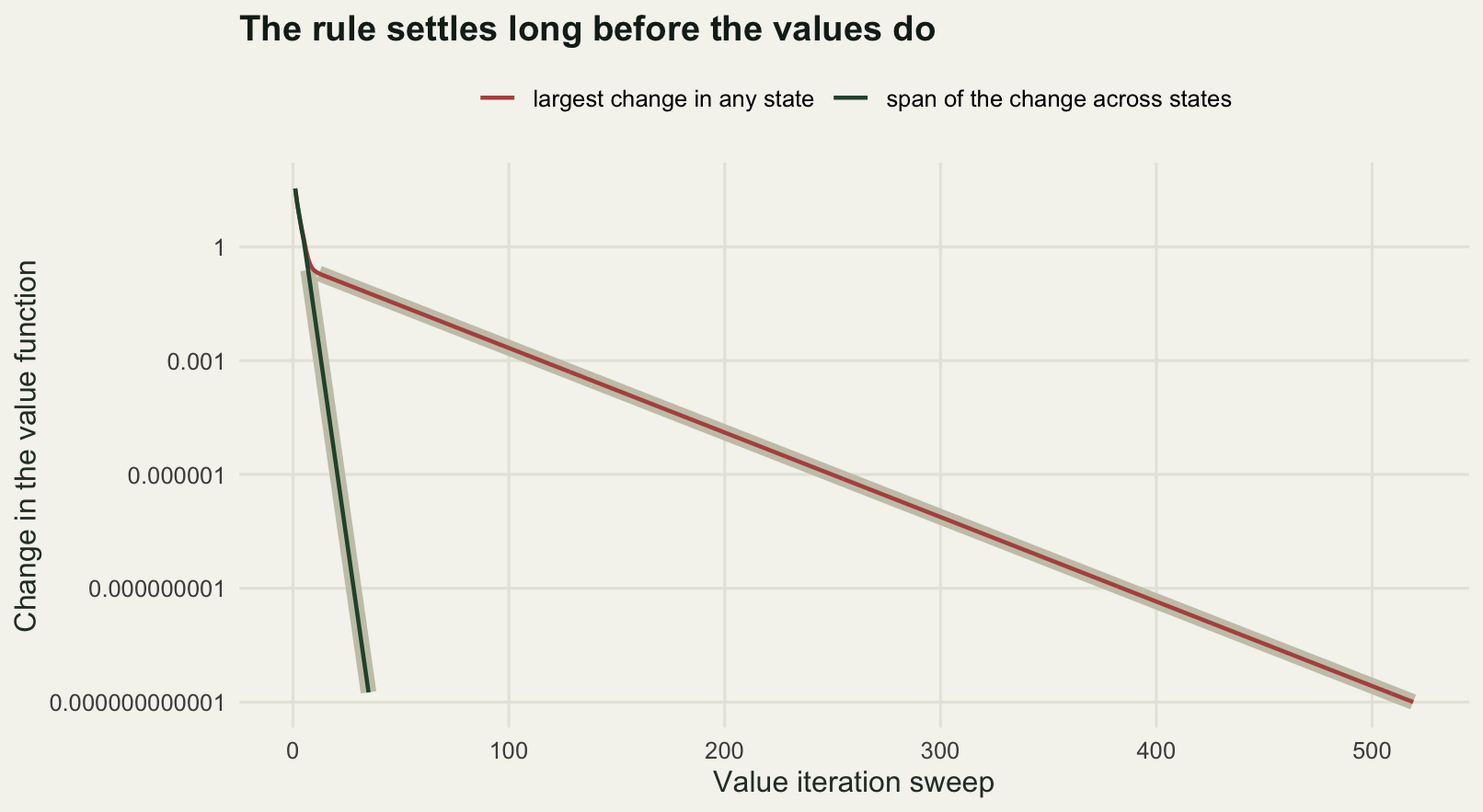
What the rule says
opt_pol <- vi$policy
j_opt <- -vi$v
q_opt <- matrix(0, n_s, n_a, dimnames = list(states, act_lab))
for (a in seq_len(n_a)) q_opt[, a] <- rew[, a] + disc * (trans[, a, ] %*% vi$v)

print(data.frame(cells = states, action = act_lab[opt_pol],
                 discounted_cost = round(j_opt, 3),
                 row.names = NULL))
cells action discounted_cost
1 0 do nothing 6.195
2 1 spot treatment 20.506
3 2 spot treatment 32.350
4 3 whole site control 42.256
5 4 whole site control 44.769
6 5 whole site control 47.199
7 6 whole site control 49.550
8 7 whole site control 51.826
9 8 whole site control 54.030
10 9 whole site control 56.164
11 10 whole site control 58.231print(round(-q_opt, 3)) do nothing spot treatment whole site control
0 6.195 7.195 34.195
1 33.973 20.506 36.972
2 52.580 32.350 39.659
3 65.208 42.931 42.256
4 75.469 52.464 44.769
5 84.401 61.144 47.199
6 92.156 69.134 49.550
7 98.801 76.567 51.826
8 104.421 83.542 54.030
9 109.117 90.138 56.164
10 112.993 96.411 58.231round(c(gap_at_three_cells = -q_opt[4, 2] + q_opt[4, 3],
gap_at_six_cells = -q_opt[7, 2] + q_opt[7, 3]), 4)gap_at_three_cells gap_at_six_cells
0.6748 19.5838 fixed_cost <- function(a) -policy_value(trans, rew, disc, rep(a, n_s))
round(rbind(optimal = j_opt, never_treat = fixed_cost(1L),
always_spot = fixed_cost(2L), always_whole_site = fixed_cost(3L)), 2) [,1] [,2] [,3] [,4] [,5] [,6] [,7] [,8]
optimal 6.19 20.51 32.35 42.26 44.77 47.20 49.55 51.83
never_treat 249.69 909.69 1019.39 1058.54 1081.98 1098.77 1111.54 1121.52
always_spot 26.35 41.05 55.21 68.80 81.81 94.23 106.08 117.36
always_whole_site 561.02 561.70 562.40 563.12 563.85 564.59 565.35 566.11
[,9] [,10] [,11]
optimal 54.03 56.16 58.23
never_treat 1129.42 1135.70 1140.70
always_spot 128.10 138.32 148.04
always_whole_site 566.89 567.68 568.47round(c(never_treat_over_optimal_at_one_cell = fixed_cost(1L)[2] / j_opt[2]), 2)never_treat_over_optimal_at_one_cell
44.36 s_opt <- stat_dist(p_opt)
round(c(share_of_years_clean = s_opt[1],
long_run_mean_cells = sum(s_opt * states),
long_run_annual_cost = sum(s_opt * (-rew[cbind(seq_len(n_s), opt_pol)]))), 4)share_of_years_clean long_run_mean_cells long_run_annual_cost
0.9673 0.0478 0.3408 The rule is short enough to put on one line. Do nothing on a clean site, send the sprayer crew at one or two invaded compartments, call the contractor at three or more. It is stationary, meaning it does not depend on the year, which is a property of the problem rather than a simplification: nothing in the transition matrix or the costs changes over time, so neither does the best response to a given state.
The discounted cost of following it is 6.195 thousand from a clean site and 42.256 from three invaded compartments. Never treating costs 909.69 from a single invaded compartment against 20.506 under the rule, a ratio of 44.36. Sending the contractor every year regardless costs 561.70 from the same start, which is cheaper than never treating but still far above what the rule pays, and is the reason a rule that responds to the state is worth computing at all.
Two numbers from the action value table set up everything that follows. At three invaded compartments, the state where the rule switches from spraying to the contractor, the two actions differ by 0.6748 thousand of discounted cost out of 42.256. At six invaded compartments the same two actions differ by 19.5838. The rule has a threshold, and at the threshold it barely matters which side of it you are on.
Followed from any starting state, the rule leaves the site clean in 0.9673 of years, at a long run average cost of 0.3408 thousand a year.
The price of a one year view
A warden who has to justify this winter’s spend from this winter’s damage will not run value iteration. She will pick the action with the smallest bill for the year ahead, which is the table printed above. That rule is not a strawman: it is what a budget cycle asks for, and it is exactly what value iteration returns when the discount factor is set to zero.
myopic_pol <- apply(rew, 1, which.max)
j_myopic <- -policy_value(trans, rew, disc, myopic_pol)
excess <- 100 * (j_myopic - j_opt) / j_opt

print(data.frame(cells = states, optimal = act_lab[opt_pol],
                 one_year = act_lab[myopic_pol],
                 cost_optimal = round(j_opt, 2), cost_one_year = round(j_myopic, 2),
                 excess_percent = round(excess, 2), row.names = NULL))
cells optimal one_year cost_optimal cost_one_year
1 0 do nothing do nothing 6.19 6.88
2 1 spot treatment spot treatment 20.51 22.98
3 2 spot treatment spot treatment 32.35 37.14
4 3 whole site control spot treatment 42.26 50.25
5 4 whole site control spot treatment 44.77 62.19
6 5 whole site control spot treatment 47.20 72.90
7 6 whole site control spot treatment 49.55 82.41
8 7 whole site control whole site control 51.83 56.16
9 8 whole site control whole site control 54.03 58.94
10 9 whole site control whole site control 56.16 61.65
11 10 whole site control whole site control 58.23 64.29
excess_percent
1 11.01
2 12.06
3 14.81
4 18.91
5 38.90
6 54.45
7 66.32
8 8.36
9 9.09
10 9.76
11 10.40round(c(mean_excess_percent = mean(excess), worst_excess_percent = max(excess),
excess_at_clean_site_percent = excess[1],
states_where_rules_differ = sum(myopic_pol != opt_pol)), 3) mean_excess_percent worst_excess_percent
23.098 66.317
excess_at_clean_site_percent states_where_rules_differ
11.012 4.000 p_myo <- t(sapply(seq_len(n_s), function(i) trans[i, myopic_pol[i], ]))
s_myo <- stat_dist(p_myo)
round(c(long_run_mean_cells_optimal = sum(s_opt * states),
long_run_mean_cells_one_year = sum(s_myo * states),
long_run_annual_cost_one_year =
sum(s_myo * (-rew[cbind(seq_len(n_s), myopic_pol)]))), 4) long_run_mean_cells_optimal long_run_mean_cells_one_year
0.0478 0.0689
long_run_annual_cost_one_year
0.3946 The one year rule sprays where the far sighted rule calls the contractor, and it does so at 4 of the eleven states, from three invaded compartments up to six. It is not lazy: it treats at every state the optimal rule treats at. It simply never buys anything whose payback takes longer than a summer.
That costs an average of 23.098 per cent in discounted cost across the eleven states, with a worst case of 66.317 per cent at six invaded compartments. From a clean site, which is where the reserve spends most of its time, the excess is 11.012 per cent.
The long run comparison is the part I did not expect. Under both rules the site is nearly always clean, and the average cover differs by almost nothing: 0.0478 compartments under the optimal rule against 0.0689 under the one year rule. The two rules leave the reserve in the same condition. The difference is in what the reserve pays on the rare occasions when the plant gets going, because the one year rule lets an outbreak run to six compartments before it escalates, and pays damage all the way up and all the way back down. Long run annual cost is 0.3408 thousand under the optimal rule and 0.3946 under the one year rule.
mdf <- data.frame(cells = states, excess = excess,
                  agree = ifelse(myopic_pol == opt_pol,
                                 "same action as the optimal rule",
                                 "different action"))

ggplot(mdf, aes(factor(cells), excess, fill = agree)) +
  geom_col(width = 0.72) +
  geom_text(aes(label = sprintf("%.0f", excess)), vjust = -0.5, size = 3.2,
            colour = te_pal$ink) +
  scale_fill_manual(values = c("different action" = te_pal$clay,
                               "same action as the optimal rule" = te_pal$sage),
                    name = NULL) +
  scale_y_continuous(limits = c(0, 76), expand = c(0, 0)) +
  labs(x = "Invaded compartments at the start", y = "Extra discounted cost (per cent)",
       title = "The one year rule costs most where it disagrees") +
  theme_te() +
  theme(legend.position = "top")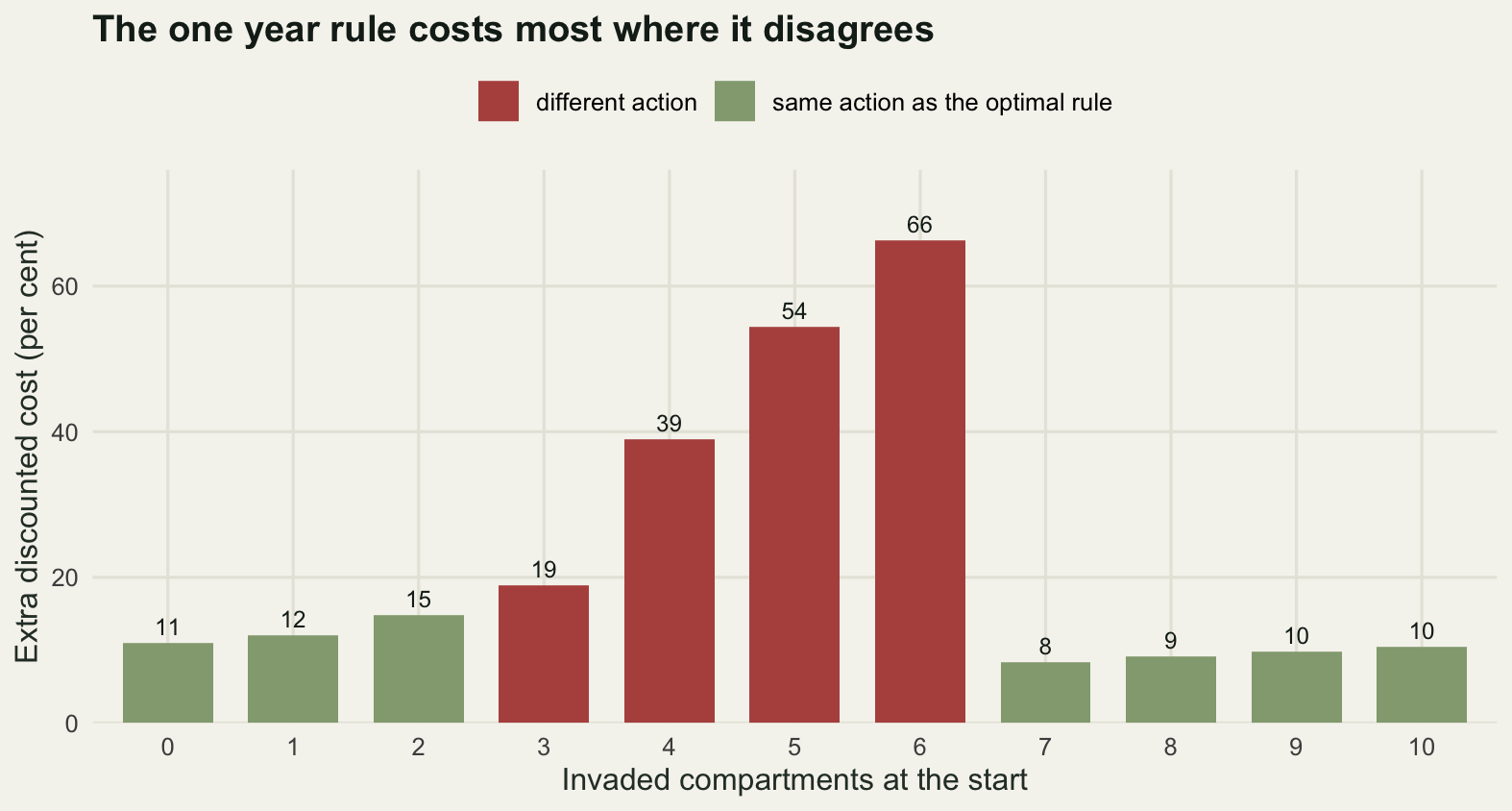
The discount factor moves the threshold, not just the total
If the one year rule is the discount factor set to zero and the rule above is the discount factor set to 0.95, then somewhere between them the rule changes, and it is worth knowing where. Sweeping the discount factor and bisecting for the exact crossings costs a few lines, because policy iteration solves each problem in a handful of sweeps.
g_grid <- seq(0, 0.995, by = 0.005)
pol_string <- function(g) paste(policy_iter(trans, rew, g)$policy, collapse = "")
sweep_pol <- sapply(g_grid, pol_string)
distinct <- unique(sweep_pol)
print(data.frame(policy = distinct,
                 escalates_at = sapply(distinct, function(s)
                   min(which(strsplit(s, "")[[1]] == "3")) - 1),
                 from = sapply(distinct, function(s) min(g_grid[sweep_pol == s])),
                 to = sapply(distinct, function(s) max(g_grid[sweep_pol == s])),
                 row.names = NULL))
policy escalates_at from to
1 12222223333 7 0.000 0.075
2 12222233333 6 0.080 0.375
3 12222333333 5 0.380 0.650
4 12223333333 4 0.655 0.920
5 12233333333 3 0.925 0.995crossing <- function(lo, hi) {
base <- pol_string(lo)
for (k in 1:50) {
mid <- (lo + hi) / 2
if (pol_string(mid) == base) lo <- mid else hi <- mid
}
(lo + hi) / 2
}
cuts <- sapply(seq_len(length(distinct) - 1), function(k)
crossing(max(g_grid[sweep_pol == distinct[k]]),
min(g_grid[sweep_pol == distinct[k + 1]])))
print(round(rbind(discount_factor = cuts,
annual_rate_percent = 100 * (1 / cuts - 1)), 3)) [,1] [,2] [,3] [,4]
discount_factor 0.077 0.375 0.650 0.922
annual_rate_percent 1192.206 166.420 53.745 8.473pol_090 <- policy_iter(trans, rew, 0.90)$policy
mis <- 100 * (-policy_value(trans, rew, disc, pol_090) - j_opt) / j_opt
round(c(discount_factor_solved_at = 0.90,
mean_cost_of_using_the_0_90_rule = mean(mis),
worst_cost_of_using_the_0_90_rule = max(mis),
states_where_it_differs = sum(pol_090 != opt_pol)), 3) discount_factor_solved_at mean_cost_of_using_the_0_90_rule
0.900 0.602
worst_cost_of_using_the_0_90_rule states_where_it_differs
2.213 1.000 Five rules over the whole range, and they differ in one place only: the number of invaded compartments at which the warden stops spraying and calls the contractor. That threshold is seven compartments for a manager who discounts everything beyond next summer, and it steps down to six, five, four and finally three as the discount factor rises. The four crossings are at discount factors 0.077, 0.375, 0.650 and 0.922, which are annual discount rates of 1192.206, 166.420, 53.745 and 8.473 per cent.
Only the last of those is a rate anyone would argue about in a meeting. Three of the four crossings sit at discount rates so severe that no public body has ever used them, and the only crossing anywhere near the range that real institutions dispute, roughly 1 to 8 per cent a year, sits just outside it at 8.473 per cent, so across that whole range the rule does not change. The discount factor is a value judgement about the future rather than a parameter of the balsam, and this measurement says what that judgement buys: not a different management philosophy, but one state’s worth of threshold.
What it costs to get it wrong is smaller still. Solving the problem at 0.90 and then living in a world that discounts at 0.95 puts the site on the wrong action at one state and costs 0.602 per cent of discounted cost on average, 2.213 per cent at the state where the two rules disagree.
grid_df <- data.frame(
  disc = rep(g_grid, each = n_s),
  cells = rep(states, length(g_grid)),
  action = factor(act_lab[as.integer(unlist(strsplit(sweep_pol, "")))],
                  levels = act_lab))

ggplot(grid_df, aes(disc, cells, fill = action)) +
  geom_tile() +
  geom_vline(xintercept = cuts[4], linetype = "dashed", colour = te_pal$ink,
             linewidth = 0.8) +
  annotate("text", x = cuts[4] - 0.02, y = 9.2, label = "8.473 per cent a year",
           hjust = 1, size = 3.2, colour = te_pal$paper) +
  scale_fill_manual(values = c(te_pal$line, te_pal$green, te_pal$forest), name = NULL) +
  scale_y_continuous(breaks = states) +
  scale_x_continuous(expand = c(0, 0)) +
  labs(x = "Discount factor", y = "Invaded compartments",
       title = "Patience moves the threshold down and leaves the shape of the rule alone") +
  theme_te() +
  theme(legend.position = "top", panel.grid = element_blank())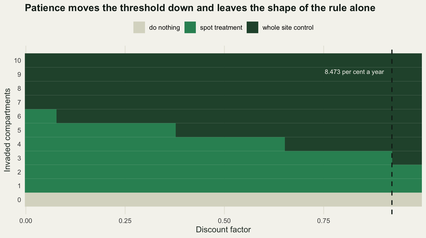
What a wrong transition matrix does
The matrix is assumed, so the last question is how much of the rule depends on the assumption. The test below multiplies every transition probability by lognormal noise with a coefficient of variation of 0.10, renormalises each row so it still sums to one, rebuilds the rewards from the perturbed matrix (the expected damage depends on the transition too), and solves the whole problem again, 200 times.
Each replicate gives two things. The perturbed model’s own answer for the discounted cost, which is what a manager working with that matrix would report. And the true cost of actually following the perturbed rule, computed by evaluating it under the original matrix. The first says how much the number moves. The second says how much the decision moves.
set.seed(20260721)
n_rep <- 200
cv_p <- 0.10
sd_log <- sqrt(log(1 + cv_p^2))

n_changed <- integer(n_rep)
changed_at <- matrix(FALSE, n_rep, n_s)
value_shift <- numeric(n_rep)
rule_loss <- numeric(n_rep)
worst_shift <- numeric(n_rep)
worst_loss <- numeric(n_rep)

for (b in seq_len(n_rep)) {
  tr_b <- trans
  for (a in seq_len(n_a)) {
    noisy <- trans[, a, ] * matrix(exp(rnorm(n_s * n_s, -sd_log^2 / 2, sd_log)),
                                   n_s, n_s)
    tr_b[, a, ] <- noisy / rowSums(noisy)
  }
  rew_b <- rewards(tr_b)
  sol_b <- policy_iter(tr_b, rew_b, disc)
  j_reported <- -sol_b$v
  j_true <- -policy_value(trans, rew, disc, sol_b$policy)
  n_changed[b] <- sum(sol_b$policy != opt_pol)
  changed_at[b, ] <- sol_b$policy != opt_pol
  value_shift[b] <- mean(100 * abs(j_reported - j_opt) / j_opt)
  worst_shift[b] <- max(100 * abs(j_reported - j_opt) / j_opt)
  rule_loss[b] <- mean(100 * (j_true - j_opt) / j_opt)
  worst_loss[b] <- max(100 * (j_true - j_opt) / j_opt)
}

c(replicates = n_rep, coefficient_of_variation = cv_p)
replicates coefficient_of_variation
200.0 0.1 print(table(states_changed = n_changed))states_changed
0 1
141 59 round(c(identical_rule = mean(n_changed == 0),
mean_states_changed = mean(n_changed),
most_states_changed = max(n_changed)), 3) identical_rule mean_states_changed most_states_changed
0.705 0.295 1.000 round(colMeans(changed_at), 3) [1] 0.000 0.000 0.000 0.295 0.000 0.000 0.000 0.000 0.000 0.000 0.000round(c(mean_value_shift_percent = mean(value_shift),
worst_state_value_shift_percent = mean(worst_shift),
mean_rule_loss_percent = mean(rule_loss),
worst_state_rule_loss_percent = mean(worst_loss),
largest_rule_loss_percent = max(rule_loss),
ratio_of_the_two = mean(value_shift) / mean(rule_loss)), 3) mean_value_shift_percent worst_state_value_shift_percent
3.527 12.439
mean_rule_loss_percent worst_state_rule_loss_percent
0.178 0.653
largest_rule_loss_percent ratio_of_the_two
0.602 19.859 In 141 of the 200 replicates the perturbed matrix returns the same rule, character for character. In the other 59 exactly one state changes action, and it is the same state every time: three invaded compartments, the threshold, where the two actions were separated by 0.6748 thousand out of 42.256. Every other state in the problem is untouched by a 10 per cent error in the transition probabilities.
The two error measures are the point of the exercise. The reported discounted cost moves by 3.527 per cent on average across states, and by 12.439 per cent in the state it moves most. The cost of acting on the perturbed rule, evaluated in the true system and averaged across states, is 0.178 per cent, and the worst any replicate reaches is 0.602 per cent, exactly the cost of the 0.90 rule above, because the perturbation moves the same threshold. The ratio of the two is 19.859: the number moves more than ten times further than the decision does.
That is not luck, and it is not specific to balsam. A rule is optimal because its action wins by some margin at each state, and a perturbation only changes the rule where that margin is small. Where the margin is small, the two actions are nearly equally good, so switching between them costs nearly nothing. The loss from an imperfectly estimated model is second order in the error, while the value estimate carries the error at first order.
The measurement also cuts the other way, and the earlier section is the counter-example. The one year rule differs from the optimal rule at six invaded compartments, where the margin is 19.5838 rather than 0.6748, and it costs 66.317 per cent there. A wrong rule near the threshold is nearly free; a wrong rule away from it is expensive. So the question to ask about a management rule is not whether it is exactly right but whether the states where it might be wrong are states where the actions are close.
pdf_df <- data.frame(
  value = c(value_shift, rule_loss),
  panel = factor(rep(c("Shift in the reported cost",
                       "True cost of following the perturbed rule"),
                     each = n_rep),
                 levels = c("Shift in the reported cost",
                            "True cost of following the perturbed rule")))
mean_df <- data.frame(
  m = c(mean(value_shift), mean(rule_loss)),
  panel = factor(levels(pdf_df$panel), levels = levels(pdf_df$panel)))

ggplot(pdf_df, aes(value)) +
  geom_histogram(bins = 34, fill = te_pal$sage, colour = te_pal$paper,
                 linewidth = 0.3) +
  geom_vline(data = mean_df, aes(xintercept = m), linetype = "dotted",
             colour = te_pal$clay, linewidth = 0.9) +
  facet_wrap(~panel) +
  labs(x = "Per cent of the optimal discounted cost", y = "Replicates",
       title = "A ten per cent error in the matrix moves the number, not the rule") +
  theme_te() +
  theme(strip.text = element_text(colour = te_pal$ink, face = "bold"))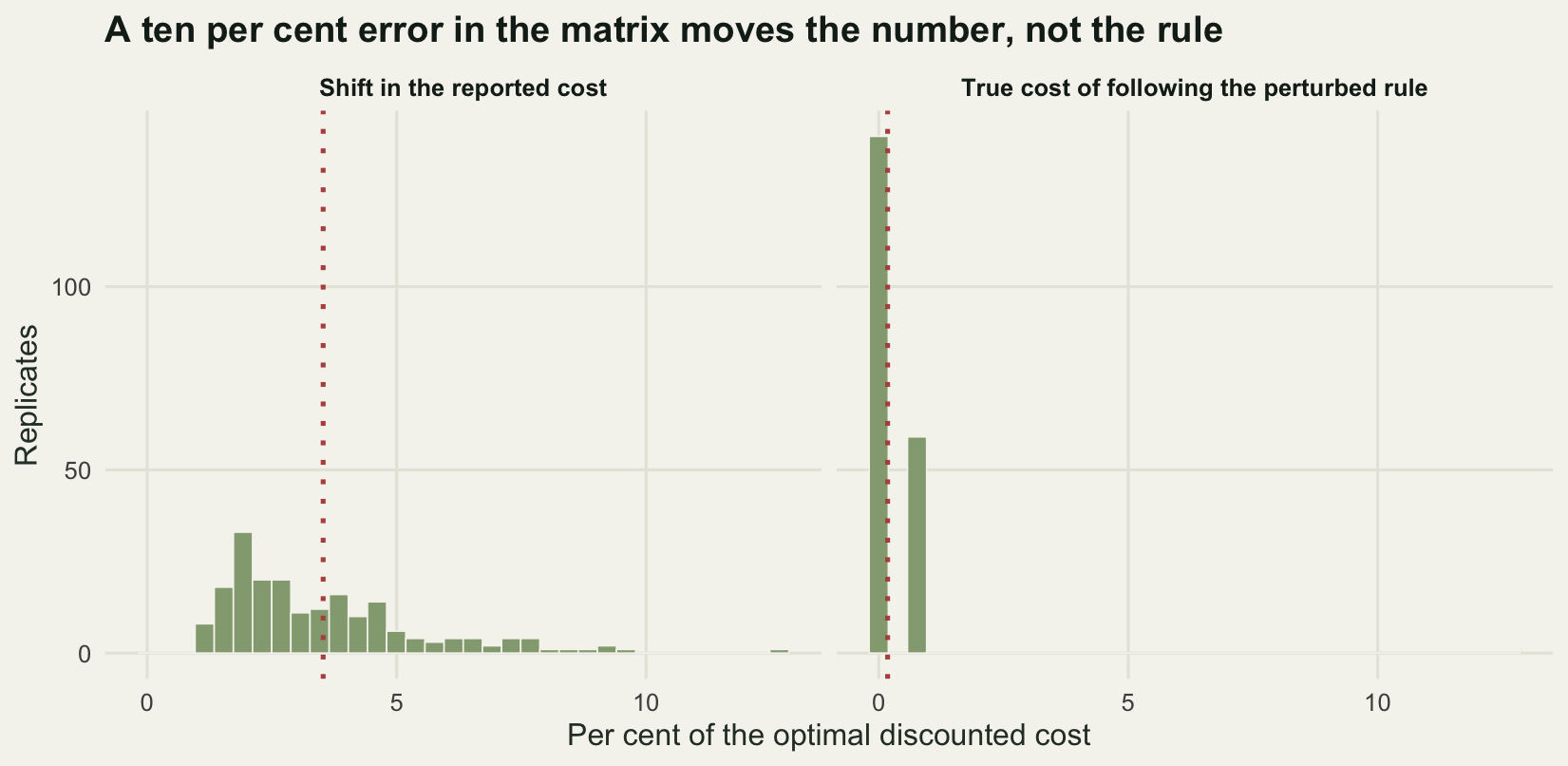
The honest limit
The perturbation test above answers a narrower question than it appears to. It asks what happens when every transition probability is wrong by a random 10 per cent, which is the kind of error you get from a finite run of observations. It says nothing about a transition matrix that is wrong in shape: a plant that spreads along a watercourse rather than between neighbours, or a seed bank that makes every clearance temporary. Structural error of that kind does move rules, and no amount of noise on the entries of the wrong matrix will reveal it. Fitting the matrix to real observations, and measuring what a short series costs, is the job of checking a sequential decision model.
Three further limits are worth stating. The state is assumed to be observed exactly every summer, and it is not: a compartment with three plants in it can be recorded as clean, which turns this into a partially observable problem with a different and much harder solution. Eleven states is a coarse grid for something that is really a continuous cover fraction, and the threshold at three compartments is only located to the nearest tenth of the reserve. And the damage exponent of 1.5, which decides how much worse full cover is than half cover, is not measured anywhere in this post; it is the value judgement that the reward function smuggles in, in the same way that weights do in a consequence table.
Where to go next
The natural next step is a state that is not a small set of boxes. Harvest problems have a continuous stock and a continuous action, the discretisation stops being a detail, and the optimal rule turns out to be a curve rather than a step, which is where stochastic dynamic programming for harvest starts. In a different direction, the question of when to stop watching a system at all is itself a sequential decision with a stopping rule, and when to stop monitoring treats it as one.
If the transition matrix is the part of this post you distrust most, that instinct is right, and adaptive management and learning is where a manager who does not know which world she is in updates her belief while acting. A state that moves and a belief that moves with it is where the ecological literature usually reaches for a dedicated package rather than a page of base R.
References
Bellman R 2010 Dynamic Programming. Princeton University Press, ISBN 978-0-691-14668-3
Puterman ML 1994 Markov Decision Processes: Discrete Stochastic Dynamic Programming. Wiley, ISBN 978-0-471-61977-2
Marescot L, Chapron G, Chades I, Fackler PL, Duchamp C, Marboutin E, Gimenez O 2013 Methods in Ecology and Evolution 4(9):872-884 (10.1111/2041-210X.12082)
Chades I, Chapron G, Cros MJ, Garcia F, Sabbadin R 2014 Ecography 37(9):916-920 (10.1111/ecog.00888)
Regan TJ, McCarthy MA, Baxter PWJ, Panetta FD, Possingham HP 2006 Ecology Letters 9(7):759-766 (10.1111/j.1461-0248.2006.00920.x)
Hanski I 1994 Journal of Animal Ecology 63(1):151-162 (10.2307/5591)