library(ggplot2)

te_pal <- list(forest = "#275139", green = "#2f8f63", sage = "#93a87f",
               clay = "#b5534e", gold = "#cda23f", line = "#dad9ca",
               ink = "#16241d", paper = "#f5f4ee")

theme_te <- function() {
  theme_minimal(base_size = 12) +
    theme(panel.grid.minor = element_blank(),
          panel.grid.major = element_line(colour = "#e7e6dc"),
          plot.background = element_rect(fill = "#f5f4ee", colour = NA),
          panel.background = element_rect(fill = "#f5f4ee", colour = NA),
          plot.title = element_text(face = "bold", colour = te_pal$ink),
          axis.title = element_text(colour = "#2c3a31"),
          axis.text = element_text(colour = "#2c3a31"))
}Implementing a plan while land is lost
R
conservation planning
decision analysis
ecology tutorial
ggplot2
A reserve plan bought two units a year for twenty years while land is cleared: the delivery gap, and the annual loss rate at which a myopic rule wins.
A regional agency has a plan. The region is a lowland mosaic of wet grassland, fen and scrub cut into a hundred and fifty planning units, each a parcel that could be bought whole. Sixty species of conservation concern have been mapped across it, and the target agreed with the funder is three occupied units for each species, or the species’ whole range where that runs to fewer than three. An analyst solved the problem once: the smallest set of units that meets every target. The map went on the wall.
Then implementation began, and implementation is slow. The agency can complete about two acquisitions a year: negotiation, valuation, board approval, and the wait for a willing seller. Forty units over twenty years is what the budget line supports, and the plan on the wall needs fewer than that, so on paper the plan is affordable and the timetable works.
While the agency buys, the rest of the region carries on. Unprotected units are drained, plough-fed, converted to maize or left to a scrub succession that nobody will pay to reverse, at some annual rate. A unit that goes is gone: it cannot be bought back, and whatever it held is no longer available to meet a target. The plan was solved on a map of the region as it stood in year zero, and by year ten that map describes a region that no longer exists.
This post measures what that does. The plan is built with greedy complementarity plus an improvement pass, exactly as the reserve selection literature builds one, and then bought over twenty years while land is cleared around it. What arrives at year twenty is set against what the plan promised, and six acquisition rules are compared under the same loss process.
Three neighbouring posts set the boundaries of this one. Complementarity and reserve selection builds the static optimum that this post spends twenty years buying, and stops when the set is chosen. Checking a conservation prioritisation names this exact failure in a single sentence of its honest limit, citing Meir, Andelman and Possingham, and then does not measure it: no schedule, no loss process, no number. That sentence is the starting point here rather than the finding. Conservation costs and return on investment is the other post in this cluster where the ranking rule, not the solver, decides the outcome, and it changes the ranking with price rather than with time.
There is also a debt to settle with the sequential decision cluster. Markov decision processes for management has a section called “The price of a one year view”, and it prices a manager’s short horizon as a tax in discounted cost. This post is the case where that tax turns into a rebate, and the quantity to find is the annual loss rate at which the sign flips.
A region, sixty species and a threat surface
The region is a fifteen by ten grid of planning units. Each species gets its own smoothed random field, thresholded at a prevalence drawn on a log scale, which gives ranges that are spatially coherent rather than scattered at random. Coherence is what makes one unit a substitute for another, and so what makes losing a unit recoverable or not.
smooth_pass <- function(z, passes) {
  nr <- nrow(z); nc <- ncol(z)
  for (k in seq_len(passes)) {
    pad <- rbind(z[1, ], z, z[nr, ])
    pad <- cbind(pad[, 1], pad, pad[, nc])
    z <- (pad[1:nr, 2:(nc + 1)] + pad[3:(nr + 2), 2:(nc + 1)] +
            pad[2:(nr + 1), 1:nc] + pad[2:(nr + 1), 3:(nc + 2)] +
            4 * pad[2:(nr + 1), 2:(nc + 1)]) / 8
  }
  z
}

smooth_field <- function(nr, nc, passes, seed, edge = 4) {
  set.seed(seed)
  z <- smooth_pass(matrix(runif((nr + 2 * edge) * (nc + 2 * edge)),
                          nr + 2 * edge, nc + 2 * edge), passes)
  z <- z[(edge + 1):(edge + nr), (edge + 1):(edge + nc)]
  (z - min(z)) / (max(z) - min(z))
}

n_row <- 15
n_col <- 10
n_units <- n_row * n_col
n_spp <- 60

set.seed(20260805)
prev_sp <- exp(runif(n_spp, log(4 / n_units), log(0.12)))
occ <- matrix(0, n_spp, n_units)
for (i in seq_len(n_spp)) {
  fld <- as.vector(smooth_field(n_row, n_col, 5, seed = 20260905 + i))
  occ[i, ] <- as.numeric(fld >= quantile(fld, 1 - prev_sp[i]))
}
occ_t <- t(occ)
rng_sp <- rowSums(occ)
tgt <- pmin(rng_sp, 3)
rich <- colSums(occ)

print(c(units = n_units, species = n_spp, range_min = min(rng_sp),
        range_median = median(rng_sp), range_max = max(rng_sp),
        occurrences_required = sum(tgt)))
units species range_min
150 60 5
range_median range_max occurrences_required
10 18 180 print(c(richness_min = min(rich), richness_median = median(rich),
richness_max = max(rich), empty_units = sum(rich == 0))) richness_min richness_median richness_max empty_units
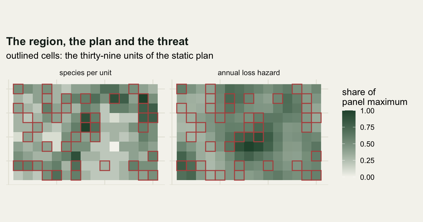
0 4 10 1 The region holds 150 units and 60 species, with ranges from 5 to 18 units and a median of 10. Every species has a target of 3 occupied units, so the plan has to deliver 180 occurrences in total. Richness runs from 0 to 10 species per unit with a median of 4, and 1 unit holds nothing at all.
The threat surface is a second smoothed field, independent of the species data, exponentiated and scaled to a mean of one. It multiplies the regional annual loss rate, so a unit on the wrong side of the region is cleared several times faster than one in the quiet corner. The regional rate is the dial that everything below is swept over.
thr_f <- as.vector(smooth_field(n_row, n_col, 5, seed = 20260806))
w_thr <- exp(1.3 * (thr_f - mean(thr_f)))
w_thr <- w_thr / mean(w_thr)

print(round(c(threat_min = min(w_thr), threat_max = max(w_thr),
              threat_ratio = max(w_thr) / min(w_thr),
              mean_multiplier = mean(w_thr)), 4))
threat_min threat_max threat_ratio mean_multiplier
0.5183 1.9018 3.6693 1.0000 print(round(c(spearman_threat_richness = cor(w_thr, rich, method = "spearman"),
spearman_threat_rarity =
cor(w_thr, colSums(occ / rng_sp), method = "spearman")), 4))spearman_threat_richness spearman_threat_rarity
0.0477 0.0252 The most threatened unit is cleared 3.67 times faster than the safest one, and the threat surface is close to independent of biodiversity value: the rank correlation between the multiplier and species richness is 0.0477. That is a deliberate choice, and it makes the test of a threat-weighted rule a fair one. Where threat and value are aligned, weighting by threat is partly a way of finding value, and the two effects cannot be separated.
Solving it once
The solver is written out here because the argument depends on knowing exactly what it does. Greedy complementarity takes, at each step, the unit that contributes the most towards targets not yet met. That rule has a known worst case: Chvatal 1979 proved the logarithmic bound for greedy set covering, which is the same problem with different words. The improvement pass runs the greedy rule many times with ties broken at random, prunes each result of units that turn out to be redundant, and keeps the smallest set found.
greedy_order <- function(short, avail, rnd = FALSE) {
  sel <- integer(0)
  sh <- short
  av <- avail
  repeat {
    need <- as.numeric(sh > 0)
    if (sum(need) == 0) break
    gn <- as.vector(need %*% occ)
    gn[!av] <- -1
    if (max(gn) <= 0) break
    cand <- which(gn == max(gn))
    k <- if (rnd && length(cand) > 1) cand[sample.int(length(cand), 1)] else cand[1]
    sel <- c(sel, k)
    av[k] <- FALSE
    sh <- pmax(0, sh - occ[, k])
  }
  sel
}

drop_redundant <- function(sel, short) {
  keep <- sel
  covr <- if (length(keep)) as.vector(occ[, keep, drop = FALSE] %*%
                                        rep(1, length(keep))) else numeric(n_spp)
  for (u in rev(sel)) if (all(pmin(covr - occ[, u], short) >= short)) {
    keep <- keep[keep != u]
    covr <- covr - occ[, u]
  }
  keep
}

best_set <- function(short, avail, n_start) {
  bs <- drop_redundant(greedy_order(short, avail), short)
  for (k in seq_len(n_start)) {
    s <- drop_redundant(greedy_order(short, avail, TRUE), short)
    if (length(s) < length(bs)) bs <- s
  }
  bs
}
Two orderings come out of the time zero solve. The plan is the improved set, worked through in the order the greedy rule builds it, most complementary unit first. Below the plan sits the rest of the region, ranked by the plain greedy order and then by richness, so the agency always has a next unit to buy even when the plan has been exhausted or destroyed.
all_open <- rep(TRUE, n_units)
ord_greedy <- greedy_order(tgt, all_open)
set.seed(4802)
set_plan <- best_set(tgt, all_open, 400)
ord_plan <- greedy_order(tgt, seq_len(n_units) %in% set_plan)
ord_tail <- setdiff(ord_greedy, ord_plan)
plan_order <- c(ord_plan, ord_tail,
                setdiff(order(rich, decreasing = TRUE), c(ord_plan, ord_tail)))
ord_thr <- c(ord_plan[order(w_thr[ord_plan], decreasing = TRUE)],
             setdiff(plan_order, ord_plan))

n_year <- 20
per_year <- 2
budget <- n_year * per_year
n_plan <- length(set_plan)
gcov <- as.vector(occ[, ord_greedy[seq_len(budget)], drop = FALSE] %*% rep(1, budget))

print(c(plain_greedy_units = length(ord_greedy), improved_plan_units = n_plan,
        greedy_excess = length(ord_greedy) - n_plan, budget_units = budget,
        years = n_year, per_year = per_year))
plain_greedy_units improved_plan_units greedy_excess budget_units
43 39 4 40
years per_year
20 2 print(round(c(plan_share_of_region_pct = 100 * n_plan / n_units,
mean_richness_in_plan = mean(rich[set_plan]),
mean_richness_region = mean(rich),
mean_threat_in_plan = mean(w_thr[set_plan])), 4))plan_share_of_region_pct mean_richness_in_plan mean_richness_region
26.0000 5.7436 4.2200
mean_threat_in_plan
0.9772 print(c(species_met_by_plan = sum(as.vector(occ[, set_plan] %*%
rep(1, n_plan)) >= tgt),
species_met_by_greedy_at_budget = sum(gcov >= tgt))) species_met_by_plan species_met_by_greedy_at_budget
60 58 Plain greedy needs 43 units to meet every target. The improvement pass finds a set of 39, which is 4 fewer, and that difference is the whole reason the static plan is worth having. The budget is 40 acquisitions, so the improved plan fits inside it with 1 to spare while the plain greedy sequence does not: truncated at 40 units it meets 58 targets out of 60.
That gap of 2 species is the value of the optimisation, and the quantity the loss process has to overturn before a myopic rule can win. The plan covers 26 per cent of the region and its units hold 5.74 species on average against 4.22 region-wide. It is not selected for safety: the mean threat multiplier inside it is 0.977, which is what independence between threat and value implies.
Twenty years of implementation
The simulation is one function with the acquisition rule as an argument. Each year the agency buys 2 units by whatever rule it follows, and then every unprotected unit that is still standing is cleared independently with its own hazard. Acquired units are safe for good; cleared units leave the problem for good.
The six rules are these. static works down the priority list fixed at year zero, skipping units that have been cleared. planthreat buys the same plan but in descending order of threat, which is the cheapest reordering a planner could apply without re-running anything. resolve re-solves the whole problem each year on the units that still exist, with the acquisitions already made locked in, and buys the first two units of the fresh plan. myopic ignores the plan and buys whatever most reduces the remaining shortfall this year. irrep buys the unit with the highest irreplaceability, weighting each unmet species by one over the number of sites still available to it, so a species whose options are disappearing pulls harder every year. threat multiplies the immediate gain by the hazard multiplier.
repair_set <- function(short, avail, keepset, n_start = 2) {
  lock <- keepset[avail[keepset]]
  sh2 <- pmax(0, short - if (length(lock)) as.vector(occ[, lock, drop = FALSE] %*%
                                                       rep(1, length(lock))) else 0)
  av2 <- avail
  av2[lock] <- FALSE
  bs <- drop_redundant(c(lock, greedy_order(sh2, av2)), short)
  for (k in seq_len(n_start)) {
    s <- drop_redundant(greedy_order(short, avail, TRUE), short)
    if (length(s) < length(bs)) bs <- s
  }
  bs
}

run_plan <- function(rule, haz, u_draw, years = n_year, rate = per_year, expo = 1) {
  acq <- rep(FALSE, n_units)
  alive <- rep(TRUE, n_units)
  got <- numeric(n_spp)
  traj <- numeric(years)
  cur <- ord_plan
  n_solve <- 0
  for (yr in seq_len(years)) {
    short <- pmax(0, tgt - got)
    avail <- alive & !acq
    if (rule == "resolve" && any(short > 0)) {
      if (!all(avail[cur])) {
        cur <- repair_set(short, avail, cur)
        n_solve <- n_solve + 1
      }
      cur <- greedy_order(short, seq_len(n_units) %in% cur)
    }
    for (k in seq_len(rate)) {
      avail <- alive & !acq
      if (!any(avail)) break
      short <- pmax(0, tgt - got)
      pick <- NA_integer_
      if (rule == "static") {
        pick <- plan_order[which(avail[plan_order])[1]]
      } else if (rule == "planthreat") {
        pick <- ord_thr[which(avail[ord_thr])[1]]
      } else if (rule == "resolve") {
        cur <- cur[avail[cur]]
        if (length(cur)) pick <- cur[1]
      } else if (any(short > 0)) {
        need <- short > 0
        occ_need <- occ_t[, need, drop = FALSE]
        gn <- as.vector(occ_need %*% rep(1, sum(need)))
        sc <- switch(rule,
                     myopic = gn,
                     threat = gn * w_thr^expo,
                     irrep = as.vector(occ_need %*%
                       (short[need] / pmax(1, colSums(occ_need * avail)))))
        sc[!avail] <- 0
        if (max(sc) > 0) pick <- which.max(sc)
      }
      if (is.na(pick)) {
        op <- which(avail)
        pick <- op[which.max(rich[op])]
      }
      acq[pick] <- TRUE
      got <- got + occ[, pick]
      if (rule == "resolve") cur <- cur[cur != pick]
    }
    open <- alive & !acq
    alive[open] <- u_draw[open, yr] >= haz[open]
    traj[yr] <- sum(got >= tgt)
  }
  left <- as.vector(occ %*% (alive & !acq))
  list(met = sum(got >= tgt), rep = sum(pmin(got, tgt)) / sum(tgt),
       unreach = sum(got + left < tgt), lost = sum(!alive),
       plan_lost = sum(!alive[set_plan]), traj = traj, solves = n_solve)
}
Two details keep the comparison fair. Every rule buys the same number of units in the same years, and a rule with nothing useful left to buy falls back on the richest unit available, so none is penalised by standing idle. And the loss draws are common random numbers: one matrix of uniforms per simulated future, shared by every rule and every loss rate, so the same clearing decisions hit each rule in the same years wherever it has not already bought the land. That pairing is what makes the differences below more precise than the spread of any single rule suggests.
The annual re-solve is allowed one shortcut that costs nothing in accuracy: if no unit of the current plan was cleared last year the plan is kept, because clearing only removes options, so a set that was the smallest feasible one last year and is still intact is still the smallest feasible one now.
rule_key <- c("static", "planthreat", "resolve", "myopic", "irrep", "threat")
rule_lab <- c("follow the static plan", "static plan, threat order",
              "re-solve every year", "largest immediate gain",
              "most irreplaceable first", "gain times threat")
p_grid <- c(0, 0.0025, 0.005, 0.0075, 0.01, 0.02, 0.03, 0.05, 0.08, 0.12)
n_rep <- 150

met <- rep_ar <- array(0, c(length(p_grid), length(rule_key), n_rep))
tj <- array(0, c(length(p_grid), length(rule_key), n_year))
extra <- array(0, c(length(p_grid), 4))
for (b in seq_len(n_rep)) {
  set.seed(61000 + b)
  u_draw <- matrix(runif(n_units * n_year), n_units, n_year)
  for (i in seq_along(p_grid)) {
    haz <- pmin(0.9, p_grid[i] * w_thr)
    for (j in seq_along(rule_key)) {
      o <- run_plan(rule_key[j], haz, u_draw)
      met[i, j, b] <- o$met
      rep_ar[i, j, b] <- o$rep
      tj[i, j, ] <- tj[i, j, ] + o$traj
      if (j == 1) extra[i, 1:3] <- extra[i, 1:3] + c(o$unreach, o$lost, o$plan_lost)
      if (j == 3) extra[i, 4] <- extra[i, 4] + o$solves
    }
  }
}
tj <- tj / n_rep
extra <- extra / n_rep
mean_met <- apply(met, 1:2, mean)
mean_rep <- apply(rep_ar, 1:2, mean)
se_met <- apply(met, 1:2, function(v) sd(v) / sqrt(n_rep))
dimnames(mean_met) <- dimnames(mean_rep) <- dimnames(se_met) <-
  list(paste(100 * p_grid), rule_key)
colnames(extra) <- c("unreachable", "units_lost", "plan_units_lost", "resolves")

at <- function(pp, rr, m = mean_met) m[match(pp, p_grid), rr]
ex_at <- function(pp, cc) extra[match(pp, p_grid), cc]

print(round(mean_met, 3))
static planthreat resolve myopic irrep threat
0 60.000 60.000 60.000 58.000 60.000 57.000
0.25 58.673 58.693 59.880 57.867 59.953 56.567
0.5 57.420 57.413 59.733 57.713 59.847 56.273
0.75 56.307 56.660 59.600 57.567 59.720 55.893
1 55.560 55.627 59.293 57.440 59.660 55.673
2 52.960 52.687 58.493 56.700 58.733 54.820
3 50.787 50.087 57.340 55.727 57.600 53.920
5 47.167 46.807 54.587 53.727 54.967 52.107
8 44.547 43.547 50.480 49.867 50.247 49.133
12 40.087 38.500 42.927 42.927 41.747 42.920print(round(cbind(loss_pct = 100 * p_grid, extra), 3)) loss_pct unreachable units_lost plan_units_lost resolves
[1,] 0.00 0.000 0.000 0.000 0.000
[2,] 0.25 0.000 6.500 0.727 0.767
[3,] 0.50 0.000 12.480 1.513 1.573
[4,] 0.75 0.013 18.380 2.307 2.507
[5,] 1.00 0.053 23.733 3.040 3.293
[6,] 2.00 0.413 42.420 5.800 6.027
[7,] 3.00 1.207 57.813 7.860 8.247
[8,] 5.00 4.213 79.933 11.480 11.907
[9,] 8.00 11.133 99.013 15.060 13.927
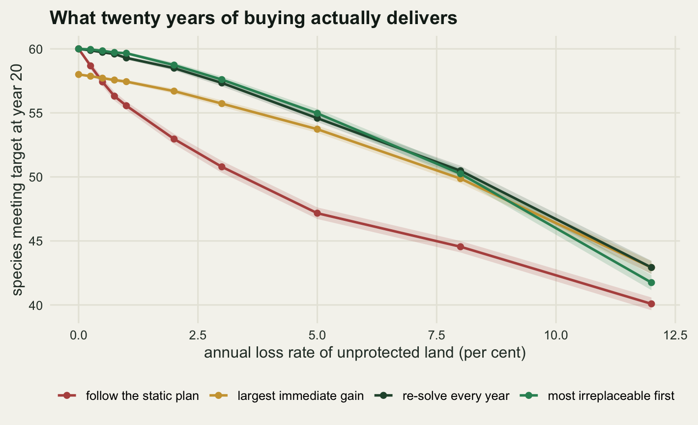
[10,] 12.00 19.747 111.000 18.393 13.673Read the first table down the static column. With no loss at all the plan delivers all 60 species, as it must. At an annual loss rate of one per cent it delivers 55.56, at two per cent 52.96, and at five per cent 47.17. The plan on the wall said sixty.
The second table says where the shortfall comes from, and it is not mostly the clearing. At a two per cent annual loss rate 42.4 of the 150 units are cleared over the twenty years, 5.8 of them from inside the plan itself. But under the static plan the number of species that no longer have enough sites left standing, bought or not, to meet the target, is 0.41. The static rule missed 7.04 targets and only 0.41 of them were beyond saving. The rest were still there, in units still standing at year twenty, unbought because the list said to buy something else.
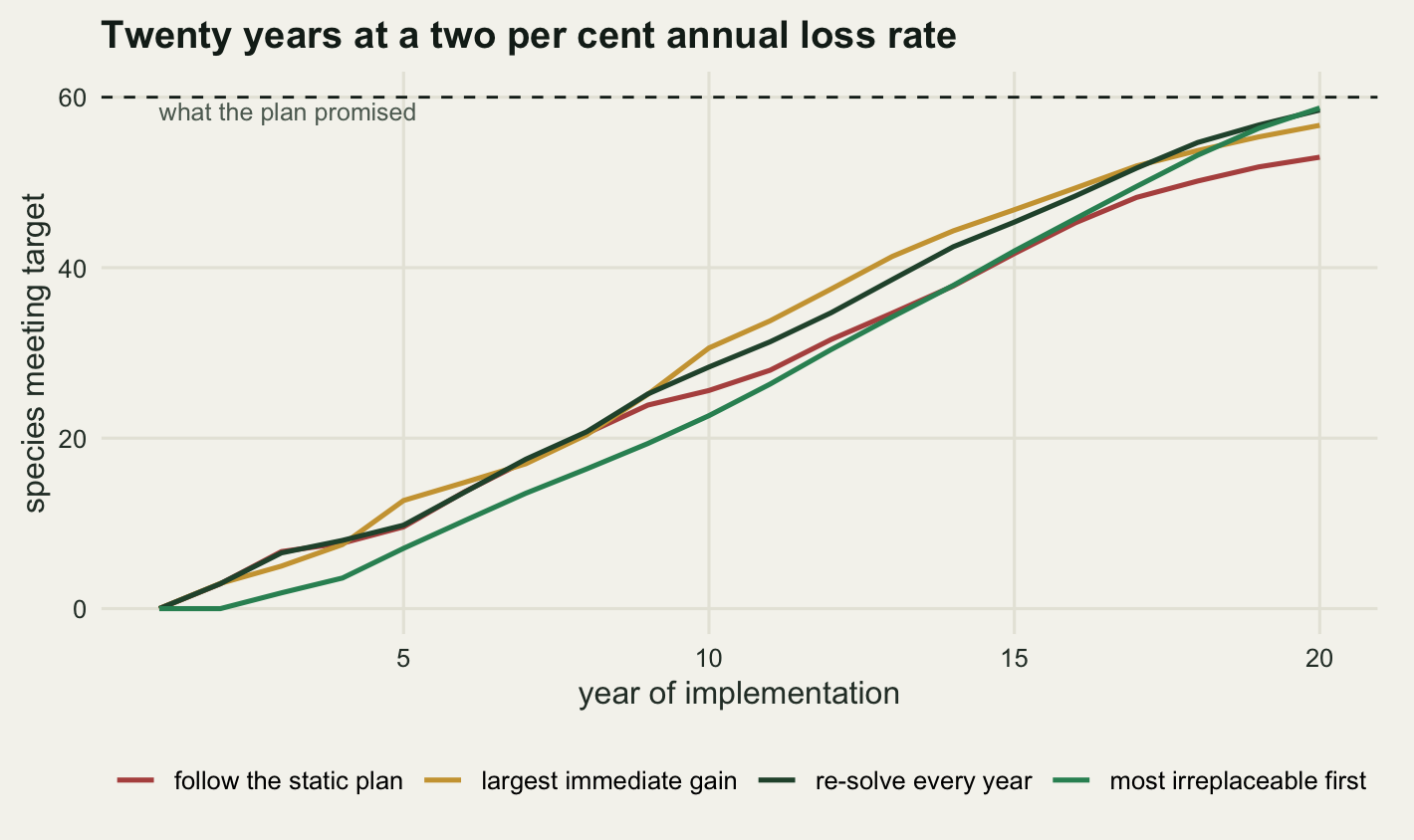
The trajectory over the twenty years is worth a look before the rules are compared at the end of them, because the interim ranking is not the final one.
i_02 <- match(0.02, p_grid)
mid_tab <- tj[i_02, , c(5, 10, 15, 20)]
dimnames(mid_tab) <- list(rule_key, paste0("year_", c(5, 10, 15, 20)))
print(round(mid_tab, 2))
year_5 year_10 year_15 year_20
static 9.59 25.59 41.65 52.96
planthreat 3.37 17.93 40.24 52.69
resolve 9.79 28.35 45.35 58.49
myopic 12.69 30.58 46.80 56.70
irrep 7.07 22.64 41.96 58.73
threat 10.94 29.39 44.89 54.82print(cbind(rank_year_10 = rank(-mid_tab[, 2]), rank_year_20 = rank(-mid_tab[, 4]))) rank_year_10 rank_year_20
static 4 5
planthreat 6 6
resolve 3 2
myopic 1 3
irrep 5 1
threat 2 4At year ten the myopic rule is comfortably ahead, with 30.58 species against 25.59 for the static plan, while the irreplaceability rule sits on 22.64, below every rule except the plan bought in threat order. Ten years later the irreplaceability rule has climbed to the top and the myopic rule has slipped to third. Buying the rarest first means buying units that complete nothing for a long time, and buying the largest immediate gain means taking the units that complete several targets at once and leaving the awkward ones for a decade in which they can be cleared. A mid-term review at year ten would put the eventual winner near the bottom of the table.
Six rules under the same futures
The sweep above ran every rule at ten loss rates on the same 150 futures. The year twenty results are the comparison the post exists for.
tab_rules <- data.frame(loss_pct = 100 * p_grid, round(mean_met, 2))
print(tab_rules, row.names = FALSE)
loss_pct static planthreat resolve myopic irrep threat
0.00 60.00 60.00 60.00 58.00 60.00 57.00
0.25 58.67 58.69 59.88 57.87 59.95 56.57
0.50 57.42 57.41 59.73 57.71 59.85 56.27
0.75 56.31 56.66 59.60 57.57 59.72 55.89
1.00 55.56 55.63 59.29 57.44 59.66 55.67
2.00 52.96 52.69 58.49 56.70 58.73 54.82
3.00 50.79 50.09 57.34 55.73 57.60 53.92
5.00 47.17 46.81 54.59 53.73 54.97 52.11
8.00 44.55 43.55 50.48 49.87 50.25 49.13
12.00 40.09 38.50 42.93 42.93 41.75 42.92print(round(cbind(loss_pct = 100 * p_grid, mean_rep), 4)) loss_pct static planthreat resolve myopic irrep threat
0 0.00 1.0000 1.0000 1.0000 0.9833 1.0000 0.9667
0.25 0.25 0.9926 0.9927 0.9993 0.9834 0.9997 0.9642
0.5 0.50 0.9853 0.9854 0.9985 0.9829 0.9991 0.9626
0.75 0.75 0.9787 0.9810 0.9978 0.9825 0.9984 0.9609
1 1.00 0.9738 0.9747 0.9960 0.9814 0.9981 0.9591
2 2.00 0.9573 0.9555 0.9909 0.9761 0.9930 0.9544
3 3.00 0.9421 0.9375 0.9839 0.9706 0.9864 0.9493
5 5.00 0.9129 0.9099 0.9652 0.9562 0.9713 0.9367
8 8.00 0.8866 0.8784 0.9324 0.9275 0.9436 0.9124
12 12.00 0.8465 0.8331 0.8690 0.8673 0.8828 0.8591print(round(cbind(loss_pct = 100 * p_grid, se_met), 4)) loss_pct static planthreat resolve myopic irrep threat
0 0.00 0.0000 0.0000 0.0000 0.0000 0.0000 0.0000
0.25 0.25 0.1333 0.1338 0.0327 0.0430 0.0173 0.0530
0.5 0.50 0.1674 0.1496 0.0470 0.0546 0.0295 0.0744
0.75 0.75 0.1772 0.1594 0.0560 0.0672 0.0414 0.0878
1 1.00 0.1661 0.1879 0.0686 0.0705 0.0525 0.0939
2 2.00 0.2040 0.2342 0.0921 0.1022 0.0977 0.0970
3 3.00 0.2364 0.2323 0.1347 0.1290 0.1233 0.1239
5 5.00 0.2304 0.2435 0.1517 0.1474 0.1725 0.1502
8 8.00 0.2285 0.2422 0.1990 0.1836 0.2208 0.1738
12 12.00 0.2543 0.3025 0.2666 0.2496 0.3018 0.2661At no loss the ordering is the one conservation planning assumes. The static plan and the annual re-solve both deliver 60 species, the irreplaceability rule also manages 60, and the myopic rule delivers 58, exactly the 2 species short that the truncated greedy sequence predicts. Weighting gain by threat is worse still at 57, because in a world with no clearing a threat weight is pure distortion.
By the time the loss rate reaches two per cent those orderings have turned over. There the static plan delivers 52.96 and the myopic rule 56.7, a difference of 3.74 species.
One rule does not turn over, and it is the cheapest fix on the list. Buying the same plan in descending order of threat delivers 52.69 against 52.96 for the plan’s own order, and at eight per cent it is 43.55 against 44.55, worse rather than better. Reordering a fixed set by urgency does not rescue it. The set was chosen on the assumption that all of it would be bought, so every member is load bearing, and hurrying to the threatened members simply changes which members are missing at the end. What has to change is the set, not the sequence.
Total representation, the second table, tells the same story in a gentler voice: the static plan reaches 95.73 per cent of the required occurrences at a two per cent loss rate against 99.09 per cent for annual re-solving. Counting occurrences hides the damage, because the targets that fail are the last one or two occurrences of species that are otherwise nearly complete, and reporting a plan as 96 per cent delivered is a much friendlier sentence than admitting 7 species missed their target.
Where the tax becomes a rebate
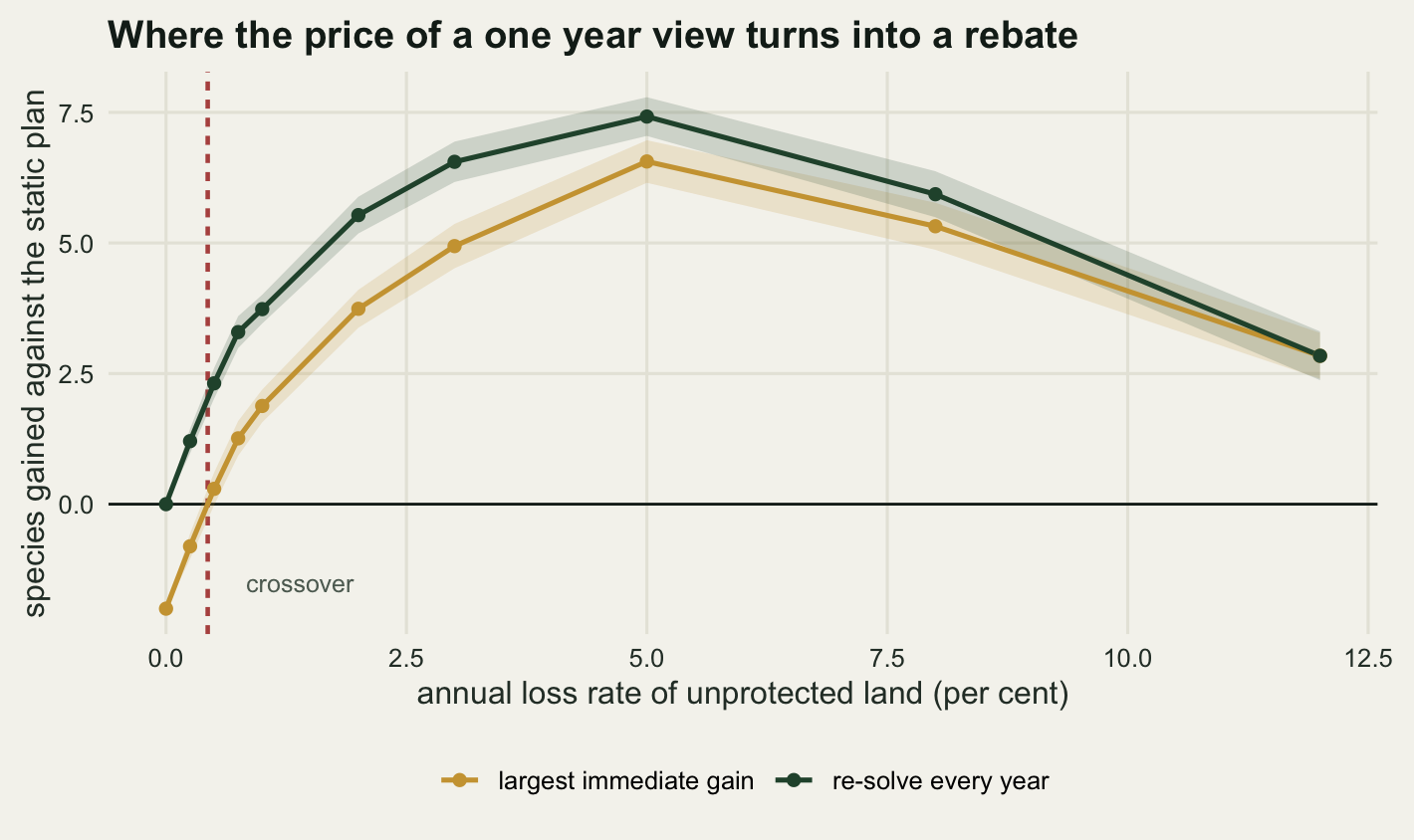
The crossing point is the number this post was written to find. Because the futures are shared, the comparison can be made replicate by replicate: for each simulated future, the species the myopic rule met minus the species the static plan met. That paired difference is -2 at a loss rate of zero, with no spread at all because nothing is random there, and it rises with the loss rate. The crossover is where it passes zero, and a bootstrap over the futures puts an interval on it.
d_my <- met[, 4, ] - met[, 1, ]
d_re <- met[, 3, ] - met[, 1, ]
d_ir <- met[, 5, ] - met[, 1, ]

cross_at <- function(dv) {
  m <- rowMeans(dv)
  i <- which(m > 0)[1]
  p_grid[i - 1] + (0 - m[i - 1]) * (p_grid[i] - p_grid[i - 1]) / (m[i] - m[i - 1])
}

set.seed(4803)
n_boot <- 2000
boot_my <- replicate(n_boot, cross_at(d_my[, sample.int(n_rep, n_rep, TRUE)]))
cross_my <- cross_at(d_my)
cross_lo <- unname(quantile(boot_my, 0.025))
cross_hi <- unname(quantile(boot_my, 0.975))

print(round(cbind(loss_pct = 100 * p_grid,
                  myopic_minus_static = rowMeans(d_my),
                  se = apply(d_my, 1, sd) / sqrt(n_rep),
                  wins = rowMeans(d_my > 0), ties = rowMeans(d_my == 0)), 4))
loss_pct myopic_minus_static se wins ties
[1,] 0.00 -2.0000 0.0000 0.0000 0.0000
[2,] 0.25 -0.8067 0.1243 0.1733 0.2133
[3,] 0.50 0.2933 0.1590 0.4200 0.2067
[4,] 0.75 1.2600 0.1693 0.6200 0.1933
[5,] 1.00 1.8800 0.1600 0.7867 0.1000
[6,] 2.00 3.7400 0.1855 0.9600 0.0267
[7,] 3.00 4.9400 0.2166 0.9667 0.0133
[8,] 5.00 6.5600 0.2078 0.9867 0.0133
[9,] 8.00 5.3200 0.2296 0.9467 0.0267
[10,] 12.00 2.8400 0.2243 0.8000 0.0867print(round(c(crossover_pct = 100 * cross_my, boot_lo_pct = 100 * cross_lo,
boot_hi_pct = 100 * cross_hi, boot_sd_pct = 100 * sd(boot_my),
boot_draws = n_boot), 4))crossover_pct boot_lo_pct boot_hi_pct boot_sd_pct boot_draws
0.4333 0.3771 0.5046 0.0332 2000.0000 print(round(c(survival_20yr_at_crossover = (1 - cross_my)^n_year,
cleared_20yr_at_crossover_pct = 100 * (1 - (1 - cross_my)^n_year),
cleared_at_2pct = 100 * (1 - 0.98^n_year)), 3)) survival_20yr_at_crossover cleared_20yr_at_crossover_pct
0.917 8.319
cleared_at_2pct
33.239 The myopic rule overtakes the static plan at an annual loss rate of 0.433 per cent, with a bootstrap interval of 0.377 to 0.505 per cent over 2000 resamples of the 150 futures. In twenty year terms that is a region losing 8.32 per cent of its unprotected land over the life of the plan.
That number is small, and its smallness is the finding. Losing under one per cent of the remaining unprotected land per year is not a crisis landscape; it is an ordinarily managed lowland region with some drainage, some ploughing and some scrub. At two per cent a year, which clears 33.2 per cent of unprotected land over twenty years, the myopic rule wins in 96 per cent of individual futures and ties in 2.7 per cent. The optimisation is not being beaten by a rare adverse draw. It is being beaten routinely.
The tax measured in the Markov decision process post came from a manager who would not look past the current budget year. The rebate here has the same source with the sign reversed. A one year view is worth something exactly when the far sighted plan is a plan about a world that will not be there, and the loss rate at which that becomes true is 0.433 per cent a year.
The rebate does not grow without limit. The paired difference peaks at 6.56 species around a loss rate of 5 per cent and falls back to 2.84 at 12 per cent. Past some point the region is being destroyed faster than any acquisition rule can respond to, and under the static plan 19.7 species no longer have enough sites left standing to reach their target. Rules stop mattering when there is nothing left to choose between.
What annual re-solving buys back
Abandoning the optimisation is not the only option, and it is not the one any agency would choose. The cheap intermediate is to keep the solver and run it again: same objective, same targets, same code, applied each year to the units that still exist. The question the brief for this post asked was how much of the myopic rule’s advantage that recovers.
gap_my <- rowMeans(d_my)
gap_re <- rowMeans(d_re)
gap_ir <- rowMeans(d_ir)
usable <- p_grid >= 0.0075
recov <- gap_re[usable] / gap_my[usable]

print(round(cbind(loss_pct = 100 * p_grid, myopic = gap_my, resolve = gap_re,
                  irreplaceable = gap_ir,
                  resolve_over_myopic = ifelse(usable, gap_re / gap_my, NA)), 4))
loss_pct myopic resolve irreplaceable resolve_over_myopic
[1,] 0.00 -2.0000 0.0000 0.0000 NA
[2,] 0.25 -0.8067 1.2067 1.2800 NA
[3,] 0.50 0.2933 2.3133 2.4267 NA
[4,] 0.75 1.2600 3.2933 3.4133 2.6138
[5,] 1.00 1.8800 3.7333 4.1000 1.9858
[6,] 2.00 3.7400 5.5333 5.7733 1.4795
[7,] 3.00 4.9400 6.5533 6.8133 1.3266
[8,] 5.00 6.5600 7.4200 7.8000 1.1311
[9,] 8.00 5.3200 5.9333 5.7000 1.1153
[10,] 12.00 2.8400 2.8400 1.6600 1.0000print(round(c(min_recovery_pct = 100 * min(recov),
max_recovery_pct = 100 * max(recov),
recovery_at_2pct = 100 * gap_re[match(0.02, p_grid)] /
gap_my[match(0.02, p_grid)],
resolve_beats_static_at_zero = gap_re[1]), 3)) min_recovery_pct max_recovery_pct
100.000 261.376
recovery_at_2pct resolve_beats_static_at_zero
147.950 0.000 print(round(cbind(loss_pct = 100 * p_grid, resolves_in_20_years = extra[, 4],
plan_units_lost = extra[, 3],
resolve_minus_myopic = gap_re - gap_my,
se = apply(d_re - d_my, 1, sd) / sqrt(n_rep)), 4)) loss_pct resolves_in_20_years plan_units_lost resolve_minus_myopic se
[1,] 0.00 0.0000 0.0000 2.0000 0.0000
[2,] 0.25 0.7667 0.7267 2.0133 0.0454
[3,] 0.50 1.5733 1.5133 2.0200 0.0659
[4,] 0.75 2.5067 2.3067 2.0333 0.0799
[5,] 1.00 3.2933 3.0400 1.8533 0.0889
[6,] 2.00 6.0267 5.8000 1.7933 0.0938
[7,] 3.00 8.2467 7.8600 1.6133 0.1098
[8,] 5.00 11.9067 11.4800 0.8600 0.1143
[9,] 8.00 13.9267 15.0600 0.6133 0.1247
[10,] 12.00 13.6733 18.3933 0.0000 0.1269It recovers all of it, and usually more. Wherever the myopic rule is ahead of the static plan the annual re-solve is ahead by at least as much: 100 to 261.4 per cent of the myopic advantage across the loss rates where the comparison is defined, and 148 per cent at a two per cent annual loss rate. It also gives up nothing at the other end: at zero loss it delivers 0 species more or fewer than the static plan, which is to say the same plan, because with nothing cleared there is never a reason to re-solve.
This was the result I expected least. The framing that produced the question, and the framing in most of the discussion of Meir, Andelman and Possingham 2004, treats re-solving as a compromise between a rigorous plan and an opportunistic one. It is not a compromise. It dominates both ends of the range, and the reason is visible in the last table: at a two per cent loss rate the plan is actually re-solved 6.03 times in 20 years, because 5.8 of its units were cleared. The rest of the time the year zero answer is still the right answer and the agency carries on down its list. Almost all of the benefit of adaptive planning comes from a handful of years in which the plan is genuinely broken and someone notices.
The irreplaceability rule is the other surprise. It carries no optimisation at all, and it matches the annual re-solve almost exactly: 58.73 species against 58.49 at two per cent, 54.97 against 54.59 at five per cent, and 60 against 60 at no loss at all. Dividing by the number of sites a species has left is doing, one purchase at a time, most of what re-solving a set cover problem does once a year. That is the same quantity the selection frequency analysis in the prioritisation post arrived at from the other direction, and it is Costello and Polasky’s dynamic reserve site selection result in a cruder form: when the future is uncertain, the site to buy now is the one whose options are closing.
Weighting by threat, and how much
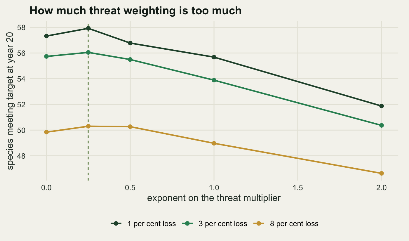
The rule that multiplies immediate gain by the hazard multiplier is the one a threat map invites, and in the sweep above it was the worst adaptive rule at every loss rate below 12 per cent. That is worth pinning down, because the failure is one of degree rather than of direction. Raising the multiplier to a power sweeps continuously from no threat weighting at all, where the rule is the myopic rule, to heavy weighting.
expo_grid <- c(0, 0.25, 0.5, 1, 2)
p_expo <- c(0.01, 0.03, 0.08)
n_rep_e <- 150
ex <- array(0, c(length(expo_grid), length(p_expo), n_rep_e))
for (b in seq_len(n_rep_e)) {
  set.seed(62000 + b)
  u_draw <- matrix(runif(n_units * n_year), n_units, n_year)
  for (i in seq_along(p_expo)) {
    haz <- pmin(0.9, p_expo[i] * w_thr)
    for (j in seq_along(expo_grid))
      ex[j, i, b] <- run_plan("threat", haz, u_draw, expo = expo_grid[j])$met
  }
}
ex_m <- apply(ex, 1:2, mean)
dimnames(ex_m) <- list(expo_grid, paste(100 * p_expo))
best_expo <- expo_grid[apply(ex_m, 2, which.max)]
d_expo <- ex[2, , ] - ex[1, , ]

print(round(ex_m, 3))
1 3 8
0 57.320 55.733 49.840
0.25 57.920 56.047 50.300
0.5 56.773 55.493 50.267
1 55.680 53.887 48.973
2 51.873 50.367 46.633print(round(rbind(best_exponent = best_expo,
gain_over_no_weighting = rowMeans(d_expo),
se = apply(d_expo, 1, sd) / sqrt(n_rep_e),
heavy_weighting_cost = ex_m[4, ] - ex_m[1, ]), 4)) 1 3 8
best_exponent 0.2500 0.2500 0.2500
gain_over_no_weighting 0.6000 0.3133 0.4600
se 0.0867 0.1171 0.1553
heavy_weighting_cost -1.6400 -1.8467 -0.8667A quarter power is the best of the five at all three loss rates, and it is worth 0.6 species at a one per cent loss rate, 0.31 at three per cent and 0.46 at eight per cent, each of them several paired standard errors from zero. Full weighting, the version a threat map suggests, costs 1.85 species at three per cent relative to ignoring threat entirely, and squaring the multiplier costs 5.37.
So threat information is worth having and worth almost nothing. Half a species out of 60, against the 6.55 species that re-solving buys at the same loss rate. The reason is in the arithmetic of the hazard: over twenty years the difference between a unit at the regional rate and a unit at 1.9 times the regional rate is a difference in survival probability, not a certainty either way, while the difference between a unit that completes three targets and a unit that completes one is a fact about the region that will not resolve itself. Threat is a tie-break. Treated as a ranking it throws away the complementarity that the whole exercise is built on, which is what the fully weighted rule does and why it loses.
The lever nobody puts in the analysis
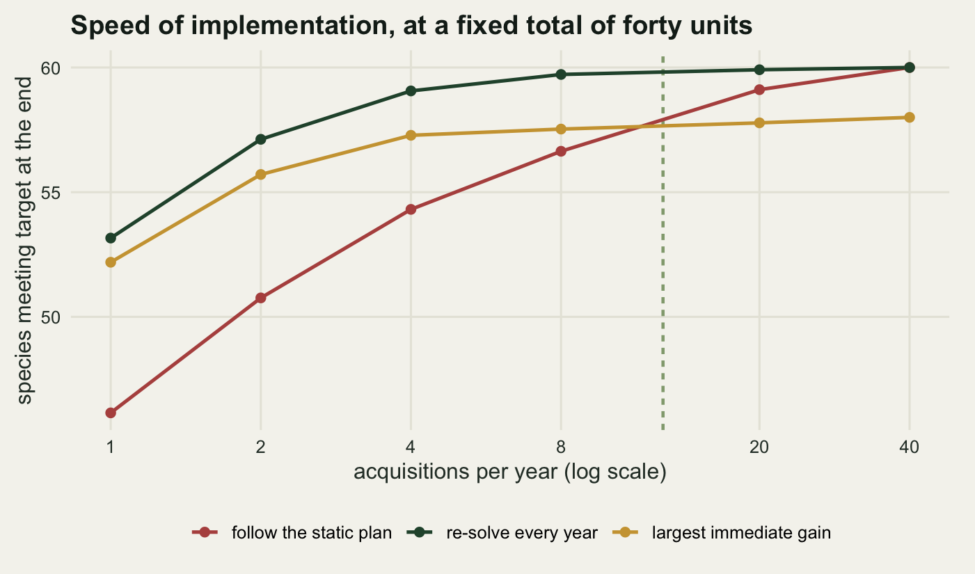
Everything above holds the acquisition rate at two units a year. That rate is not a fact of nature; it is a budget, a staffing level and a legal process. Holding the total at 40 units and varying how fast they are bought separates the effect of implementation speed from the effect of the budget, and it asks the question the other way round: how quickly would the agency have to move before the plan on the wall is worth following?
rate_grid <- c(1, 2, 4, 8, 20, 40)
rate_key <- c("static", "resolve", "myopic")
n_rep_r <- 100
ra <- array(0, c(length(rate_grid), 3, n_rep_r))
for (b in seq_len(n_rep_r)) {
  set.seed(63000 + b)
  u_draw <- matrix(runif(n_units * 40), n_units, 40)
  haz <- pmin(0.9, 0.03 * w_thr)
  for (i in seq_along(rate_grid)) for (j in seq_along(rate_key))
    ra[i, j, b] <- run_plan(rate_key[j], haz, u_draw,
                            years = budget / rate_grid[i], rate = rate_grid[i])$met
}
ra_m <- apply(ra, 1:2, mean)
dimnames(ra_m) <- list(rate_grid, rate_key)
d_rate <- rowMeans(ra[, 1, ] - ra[, 3, ])
i_rc <- which(d_rate > 0)[1]
rate_cross <- rate_grid[i_rc - 1] + (0 - d_rate[i_rc - 1]) *
  (rate_grid[i_rc] - rate_grid[i_rc - 1]) / (d_rate[i_rc] - d_rate[i_rc - 1])

print(round(cbind(units_per_year = rate_grid, years_to_finish = budget / rate_grid,
                  ra_m, static_minus_myopic = d_rate,
                  se = apply(ra[, 1, ] - ra[, 3, ], 1, sd) / sqrt(n_rep_r)), 3))
units_per_year years_to_finish static resolve myopic static_minus_myopic
1 1 40 46.15 53.16 52.19 -6.04
2 2 20 50.76 57.12 55.71 -4.95
4 4 10 54.31 59.06 57.28 -2.97
8 8 5 56.64 59.72 57.53 -0.89
20 20 2 59.11 59.91 57.78 1.33
40 40 1 60.00 60.00 58.00 2.00
se
1 0.206
2 0.249
4 0.215
8 0.188
20 0.120
40 0.000print(round(c(rate_crossover_units_per_year = rate_cross,
years_at_crossover = budget / rate_cross,
static_at_2_per_year = ra_m["2", "static"],
static_at_8_per_year = ra_m["8", "static"],
resolve_at_1_per_year = ra_m["1", "resolve"]), 3))rate_crossover_units_per_year years_at_crossover
12.811 3.122
static_at_2_per_year static_at_8_per_year
50.760 56.640
resolve_at_1_per_year
53.160 At a three per cent annual loss rate the static plan overtakes the myopic rule at 12.81 acquisitions a year, which is the whole 40 unit budget spent in 3.12 years. Below that speed the plan on the wall is the wrong document. Two acquisitions a year delivers 50.76 species under the static plan and eight a year delivers 56.64, so quadrupling the pace of implementation is worth 5.88 species: about the same as the 6.36 that re-solving buys at the original pace, and considerably harder to arrange.
There is a second reading of that table for an agency that cannot go faster. Re-solving every year at one acquisition a year, the slowest schedule tested, delivers 53.16 species, more than the static plan manages at twice that speed (50.76) and not far short of what it manages at four times (54.31). Rethinking the plan substitutes for a good deal of money, and it is the cheaper of the two.
The honest limit
The loss process here is the weakest part of the model and it is weak in a direction that flatters every adaptive rule. Clearing is independent between units and between years, with a hazard that never changes. Real conversion is contagious: a drainage scheme takes a block, a road opens a district, a change in subsidy moves a whole region at once. Correlated loss would take out several units of a plan in the same year, which makes re-solving more valuable, but it would also destroy the alternatives that the adaptive rules rely on finding, and which of those dominates is not something this simulation can answer. Visconti, Pressey, Segan and Wintle 2010 model spatially structured threat directly and find that the design consequences depend on the spatial pattern of the threat, not only its rate.
The hazard is also assumed known. The threat-weighted rules here were handed the exact multiplier that generates the clearing, which no agency has; a real threat layer is a model output with its own error. Since the best exponent measured was 0.25 and the gain at that exponent was 0.31 species, there is not much for the error to eat, and the practical conclusion, that threat belongs in the tie-break rather than in the ranking, is not sensitive to it.
Every target here is a count of occupied units, which is the convention the whole minimum set literature runs on and the one Margules and Pressey 2000 set out. It is not persistence. Cabeza and Moilanen 2001 make the distinction that matters for this post specifically: a unit that is bought is treated here as safe for ever and as contributing its species for ever, which converts an ecological question about population viability into an accounting question about ownership. If protected units can still lose species, the static plan’s problem gets worse rather than better, because it front-loads a set chosen without regard to what happens after purchase.
The plan is solved by a heuristic, so none of the sets here is proven optimal. The improvement pass found 39 units against plain greedy’s 43, and a proper integer programme would very likely find fewer. A smaller static plan would leave more of the budget spare, which would push the crossover to a higher loss rate. The direction of that bias is known, its size is not, and it is the one number in this post that a better solver could move.
The comparison also gives the static rule no credit for a property it really has. A plan fixed at year zero can be published, funded, defended in front of a board and audited afterwards, and a rule that changes its mind every year cannot. Pressey, Cabeza, Watts, Cowling and Wilson 2007 treat that gap between a plan and its implementation as the central problem of the field. The measurements above say what the fixed document costs in species, not what it buys in institutional weight.
Where to go next
The result that keeps its shape across everything above is that the schedule is part of the plan. Wilson, McBride, Bode and Possingham 2006 made that argument for global conservation investment: the order in which money is spent changes the outcome as much as which places it is spent on. What this post adds is a price for ignoring it in one region, and the price is paid at loss rates far lower than the ones that make the case for planning in the first place.
Two threads lead out of it. The first is the sequential decision cluster, which poses the same problem as a state that moves under an action and solves it rather than comparing rules; a hundred and fifty units is where dynamic programming stops being possible and heuristics of the kind used here become the only option. The second is the irreplaceability result: a per purchase score, needing no solver, matched a full annual re-optimisation at every loss rate below 12 per cent and fell behind it only at the top of the sweep, so what breaks the equivalence there is worth knowing before recommending it to anybody.
References
Margules CR, Pressey RL 2000 Nature 405(6783):243-253 (10.1038/35012251)
Chvatal V 1979 Mathematics of Operations Research 4(3):233-235 (10.1287/moor.4.3.233)
Cabeza M, Moilanen A 2001 Trends in Ecology and Evolution 16(5):242-248 (10.1016/S0169-5347(01)02125-5)
Meir E, Andelman S, Possingham HP 2004 Ecology Letters 7(8):615-622 (10.1111/j.1461-0248.2004.00624.x)
Costello C, Polasky S 2004 Resource and Energy Economics 26(2):157-174 (10.1016/j.reseneeco.2003.11.005)
Wilson KA, McBride MF, Bode M, Possingham HP 2006 Nature 440(7082):337-340 (10.1038/nature04366)
Pressey RL, Cabeza M, Watts ME, Cowling RM, Wilson KA 2007 Trends in Ecology and Evolution 22(11):583-592 (10.1016/j.tree.2007.10.001)
Visconti P, Pressey RL, Segan DB, Wintle BA 2010 Biological Conservation 143(3):756-767 (10.1016/j.biocon.2009.12.018)