Complementarity and reserve selection

Compare hotspot and greedy complementarity reserve selection in base R, and measure how many planning units each rule needs to represent every species.

The intuitive way to choose protected areas is to rank sites by how many species they hold and work down the list. It is easy to explain, it produces a defensible map, and it is wrong often enough to matter. The reason is that species-rich sites tend to hold the same species as each other, so the second site on the list adds much less than its species count suggests.

The quantity that matters is not richness but complementarity: what a site adds to the set you have already chosen (Kirkpatrick 1983, Vane-Wright et al 1991, Pressey et al 1993). This tutorial builds a synthetic planning region in base R, implements three selection rules by hand, and measures how many planning units each rule needs before every species appears at least once.

A region and its species

The region is a 20 by 20 grid of planning units. Each species gets a smooth random field of its own, thresholded at a prevalence drawn on a log scale so that ranges run from a handful of units to about a third of the region. Thresholding a smoothed field rather than scattering occurrences at random is what makes the ranges spatially coherent, which is the property the whole problem depends on.

library(ggplot2)

te_pal <- list(forest = "#275139", green = "#2f8f63", sage = "#93a87f",
               clay = "#b5534e", gold = "#cda23f", line = "#dad9ca",
               ink = "#16241d", paper = "#f5f4ee")

theme_te <- function() {
  theme_minimal(base_size = 12) +
    theme(panel.grid.minor = element_blank(),
          panel.grid.major = element_line(colour = "#e7e6dc"),
          plot.background = element_rect(fill = "#f5f4ee", colour = NA),
          panel.background = element_rect(fill = "#f5f4ee", colour = NA),
          plot.title = element_text(face = "bold", colour = te_pal$ink),
          axis.title = element_text(colour = "#2c3a31"))
}

smooth_field <- function(n, passes, seed) {
  set.seed(seed)
  z <- matrix(runif(n * n), n, n)
  for (p in seq_len(passes)) {
    pad <- rbind(z[1, ], z, z[n, ])
    pad <- cbind(pad[, 1], pad, pad[, n])
    z <- (pad[1:n, 2:(n + 1)] + pad[3:(n + 2), 2:(n + 1)] +
            pad[2:(n + 1), 1:n] + pad[2:(n + 1), 3:(n + 2)] +
            4 * pad[2:(n + 1), 2:(n + 1)]) / 8
  }
  (z - min(z)) / (max(z) - min(z))
}

side <- 20
n_units <- side * side
n_spp <- 80

set.seed(4801)
prevalence <- exp(runif(n_spp, log(3 / n_units), log(1 / 3)))

pa <- matrix(FALSE, n_spp, n_units)
for (i in seq_len(n_spp)) {
  big <- smooth_field(side + 8, 4, seed = 5200 + i)
  fld <- as.vector(big[5:(side + 4), 5:(side + 4)])
  pa[i, ] <- fld >= quantile(fld, 1 - prevalence[i])
}
range_size <- rowSums(pa)
richness <- colSums(pa)

cat("grid side:", side, " field generated at side:", side + 8, "\n")

grid side: 20  field generated at side: 28 

cat("planning units:", n_units, " species:", n_spp, "\n")

planning units: 400  species: 80 

cat("range size: smallest", min(range_size), " median", median(range_size),
    " largest", max(range_size), "\n")

range size: smallest 4  median 30  largest 131 

cat("range size quantiles (units occupied):\n")

range size quantiles (units occupied):

print(quantile(range_size, c(0, 0.25, 0.5, 0.75, 1)))

    0%    25%    50%    75%   100% 
  4.00  11.75  30.00  63.50 131.00 

cat("species in 10 units or fewer:", sum(range_size <= 10), "\n")

species in 10 units or fewer: 18 

cat("richness per unit quantiles:\n")

richness per unit quantiles:

print(quantile(richness, c(0, 0.25, 0.5, 0.75, 1)))

  0%  25%  50%  75% 100% 
   1    6    8   10   16 

cat("mean richness per unit:", round(mean(richness), 2), "\n")

mean richness per unit: 7.94 

Range sizes run from 4 units to 131, with a median of 30, and 18 of the 80 species occupy 10 units or fewer. Richness per unit runs from 1 to 16 with a median of 8 and a mean of 7.94. Nothing about the region is unusual: it is the ordinary situation in which a few places are rich, most species are moderately widespread, and a minority are confined to one or two patches.

The field is generated on a 28 by 28 grid and the central 20 by 20 block is kept. Smoothing with replicated edges inflates the values at the boundary, so thresholding a field generated at the working size puts a systematic excess of occurrences along the edge of the map. Cropping removes the artefact, and it is worth checking for whenever a simulated range map is built this way.

Three rules for choosing units

Each rule is a function returning the order in which the 400 units are selected, so the same downstream code can score all three. The scoring machinery is one step: for every species, find the position in the ordering at which it is first covered, then accumulate.

first_step <- function(ord, pa) {
  pos <- integer(length(ord))
  pos[ord] <- seq_along(ord)
  apply(pa, 1, function(occ) min(pos[occ]))
}

rep_curve <- function(ord, pa) {
  cumsum(tabulate(first_step(ord, pa), nbins = length(ord)))
}

order_richness <- function(pa) {
  order(colSums(pa), decreasing = TRUE)
}

order_greedy <- function(pa, range_size) {
  nu <- ncol(pa)
  covered <- rep(FALSE, nrow(pa))
  chosen <- integer(0)
  left <- seq_len(nu)
  repeat {
    if (length(left) == 0) break
    if (all(covered)) {
      chosen <- c(chosen, left[order(colSums(pa[, left, drop = FALSE]),
                                     decreasing = TRUE)])
      break
    }
    avail <- pa[!covered, left, drop = FALSE]
    gain <- colSums(avail)
    rar <- colSums(avail * (1 / range_size[!covered]))
    tie <- which(gain == max(gain))
    k <- tie[which.max(rar[tie])]
    chosen <- c(chosen, left[k])
    covered <- covered | pa[, left[k]]
    left <- left[-k]
  }
  chosen
}

Richness-first fixes the whole order at the start, which is the point: a hotspot ranking is computed once and never updated as sites are added. Greedy complementarity recomputes at every step, choosing the unit that adds the most so far unrepresented species. Ties on that count are broken by the summed inverse range size of the species added, so when two units both add three new species the one whose species are more restricted wins; remaining ties go to the lower unit index. Once everything is represented the greedy rule has nothing left to optimise, so the remaining units are appended in decreasing richness order and the curve is flat there anyway.

The third rule is random order, replicated, which is the baseline that tells you how much of any rule’s performance is just the arithmetic of covering 80 clustered ranges with 400 units.

ord_rich <- order_richness(pa)
ord_greedy <- order_greedy(pa, range_size)
cur_rich <- rep_curve(ord_rich, pa)
cur_greedy <- rep_curve(ord_greedy, pa)

set.seed(4802)
n_rep <- 200
rand_mat <- replicate(n_rep, rep_curve(sample(n_units), pa))

need <- function(cur, target) which(cur >= target)[1]
u_rich <- need(cur_rich, n_spp)
u_greedy <- need(cur_greedy, n_spp)
rand_full <- apply(rand_mat, 2, need, target = n_spp)

cat("units for complete representation: complementarity", u_greedy,
    " richness-first", u_rich, "\n")

units for complete representation: complementarity 17  richness-first 165 

cat("random order over", n_rep, "replicates: mean",
    round(mean(rand_full), 2), " range", min(rand_full), "to",
    max(rand_full), "\n")

random order over 200 replicates: mean 187.72  range 73 to 334 

cat("saving of complementarity over richness-first:",
    round(100 * (1 - u_greedy / u_rich), 1), "percent\n")

saving of complementarity over richness-first: 89.7 percent

cat("share of the region needed: complementarity",
    round(100 * u_greedy / n_units, 2), "percent  richness-first",
    round(100 * u_rich / n_units, 2), "percent\n")

share of the region needed: complementarity 4.25 percent  richness-first 41.25 percent

Complementarity represents all 80 species in 17 units. Richness-first needs 165. Random order needs 187.72 units on average, with individual replicates between 73 and 334. That is a saving of 89.7 percent, or in area terms 4.25 percent of the region against 41.25 percent.

The result that should give the hotspot approach pause is not the gap between complementarity and random. It is that richness-first, a rule built entirely out of biodiversity information, performs no better than picking units out of a hat: 165 against a random mean of 187.72, well inside the random spread.

Representation at a fixed budget

Complete representation is a target, not a budget. Planning usually runs the other way: a fixed number of units is available and the question is what fraction of the biota they cover.

budget_row <- function(b) {
  data.frame(units = b,
             complementarity = cur_greedy[b],
             richness_first = cur_rich[b],
             random_mean = round(mean(rand_mat[b, ]), 2),
             random_min = min(rand_mat[b, ]),
             random_max = max(rand_mat[b, ]))
}
tab_budget <- rbind(budget_row(15), budget_row(30))
print(tab_budget, row.names = FALSE)

 units complementarity richness_first random_mean random_min random_max
    15              78             62       50.69         43         61
    30              80             72       62.67         54         71

cat("as percentages of", n_spp, "species:\n")

as percentages of 80 species:

print(data.frame(units = tab_budget$units,
                 complementarity = round(100 * tab_budget$complementarity / n_spp, 1),
                 richness_first = round(100 * tab_budget$richness_first / n_spp, 1),
                 random_mean = round(100 * tab_budget$random_mean / n_spp, 1)),
      row.names = FALSE)

 units complementarity richness_first random_mean
    15            97.5           77.5        63.4
    30           100.0           90.0        78.3

At 15 units complementarity holds 78 species and richness-first holds 62, which is 97.5 percent against 77.5 percent; the random mean is 50.69 species, or 63.4 percent. At 30 units complementarity is complete at 80 species and richness-first has reached 72, or 90 percent. The gap is largest exactly where planning budgets sit, in the range where a rule has to be selective.

map_df <- data.frame(x = rep(seq_len(side), each = side),
                     y = rep(seq_len(side), times = side),
                     richness = richness)
pick_df <- rbind(
  data.frame(x = ((ord_rich[1:15] - 1) %/% side) + 1,
             y = ((ord_rich[1:15] - 1) %% side) + 1,
             rule = "richness-first, first 15 units"),
  data.frame(x = ((ord_greedy[1:15] - 1) %/% side) + 1,
             y = ((ord_greedy[1:15] - 1) %% side) + 1,
             rule = "complementarity, first 15 units"))
pick_df$rule <- factor(pick_df$rule,
                       levels = c("richness-first, first 15 units",
                                  "complementarity, first 15 units"))
map_both <- do.call(rbind, lapply(levels(pick_df$rule), function(z)
  data.frame(map_df, rule = factor(z, levels = levels(pick_df$rule)))))

ggplot(map_both, aes(x, y)) +
  geom_raster(aes(fill = richness)) +
  geom_tile(data = pick_df, fill = NA, colour = te_pal$clay,
            linewidth = 0.8) +
  facet_wrap(~rule) +
  coord_equal() +
  scale_fill_gradient(low = te_pal$paper, high = te_pal$forest,
                      name = "species") +
  labs(title = "The same region, two selection rules",
       subtitle = "outlined cells are the first 15 units each rule selects",
       x = NULL, y = NULL) +
  theme_te() +
  theme(axis.text = element_blank(), panel.grid = element_blank())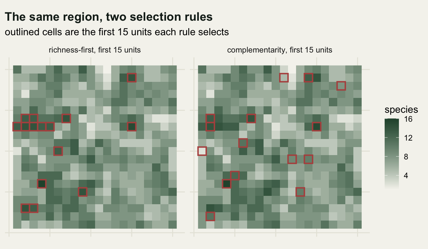

Figure 1: Species richness per planning unit in the simulated region, with the first 15 units chosen by richness-first and by greedy complementarity outlined.

Why the richest units are the wrong answer

The map already shows the mechanism: the richness-first picks sit inside the same few dark patches. Putting a number on that similarity is the point of the next block. Jaccard similarity on the species lists of two units is the shared species divided by the species in either.

jac <- function(u, v) sum(pa[, u] & pa[, v]) / sum(pa[, u] | pa[, v])
mean_pair <- function(units) {
  cmb <- combn(units, 2)
  mean(apply(cmb, 2, function(z) jac(z[1], z[2])))
}

cat("mean pairwise Jaccard, 10 richest units:",
    round(mean_pair(ord_rich[1:10]), 4),
    " first 10 complementarity picks:",
    round(mean_pair(ord_greedy[1:10]), 4), "\n")

mean pairwise Jaccard, 10 richest units: 0.1878  first 10 complementarity picks: 0.0741 

cat("10 richest units: occurrences", sum(richness[ord_rich[1:10]]),
    " distinct species", sum(rowSums(pa[, ord_rich[1:10]]) > 0), "\n")

10 richest units: occurrences 141  distinct species 58 

cat("first 10 complementarity picks: occurrences",
    sum(richness[ord_greedy[1:10]]),
    " distinct species", sum(rowSums(pa[, ord_greedy[1:10]]) > 0), "\n")

first 10 complementarity picks: occurrences 114  distinct species 71 

fs_rich <- first_step(ord_rich, pa)
cat("species still missing from the richness-first set at 50 units:",
    sum(fs_rich > 50), " at 100 units:", sum(fs_rich > 100), "\n")

species still missing from the richness-first set at 50 units: 4  at 100 units: 1 

rank_rich <- rank(-richness, ties.method = "min")
cat("richness rank of each of the first 17 complementarity picks:\n")

richness rank of each of the first 17 complementarity picks:

print(as.vector(rank_rich[ord_greedy[1:u_greedy]]))

 [1]   1   3   9   2  43 104  22 330 161  43  70   9 394   3  70  70 104

cat("of those 17 units,", sum(rank_rich[ord_greedy[1:u_greedy]] > 40),
    "fall outside the 40 richest units\n")

of those 17 units, 10 fall outside the 40 richest units

worst <- ord_greedy[which.max(rank_rich[ord_greedy[1:u_greedy]])]
cat("poorest unit the rule selects: richness rank", rank_rich[worst],
    " species present", richness[worst],
    " smallest range among them", min(range_size[pa[, worst]]), "\n")

poorest unit the rule selects: richness rank 394  species present 2  smallest range among them 4 

The 10 richest units share a mean Jaccard similarity of 0.1878; the first 10 complementarity picks share 0.0741, less than half as much. The consequence is in the next two lines. The 10 richest units contain 141 occurrences but only 58 distinct species. The first 10 complementarity picks contain fewer occurrences, 114, and more species, 71. Selecting for richness buys records; selecting for complementarity buys species.

Extending the richness ranking does not fix the problem. At 50 units, an eighth of the region, 4 species have still never appeared in the richness-first set, and one species is still missing at 100 units. Those species live outside the rich patches, and no amount of working down the ranking reaches them until the ranking runs out of rich units.

The complementarity ordering goes the other way. Of the 17 units it needs, 10 are outside the 40 richest, and the poorest is ranked 394th of 400 with only 2 species in it. It is selected because one of those two species occupies 4 units in the whole region and lives nowhere else that has been chosen. A ranking by richness would reach that unit near the end of the list, if at all.

The representation curve

Species represented against units selected is the curve the reserve selection literature is built on (Csuti et al 1997). Reading three targets off it is the usual summary.

target_row <- function(fr) {
  tg <- ceiling(fr * n_spp)
  data.frame(target_pct = 100 * fr,
             species = tg,
             complementarity = need(cur_greedy, tg),
             richness_first = need(cur_rich, tg),
             random_mean = round(mean(apply(rand_mat, 2, need, target = tg)), 2))
}
tab_target <- rbind(target_row(0.5), target_row(0.9), target_row(1))
print(tab_target, row.names = FALSE)

 target_pct species complementarity richness_first random_mean
         50      40               4              4        9.07
         90      72              11             30       58.92
        100      80              17            165      187.72

Halfway is easy and the rules are indistinguishable: 4 units each. At 90 percent representation complementarity needs 11 units and richness-first needs 30. At 100 percent the ratio has gone to 17 against 165. The rules diverge in the tail, because the tail is made of restricted-range species and those are exactly what a richness ranking cannot see.

That shape has a practical reading. A hotspot map is a perfectly reasonable way to protect the commonest two thirds of a biota, and it is a bad way to protect the rest. Since the rest is usually what the protection is for, the choice of rule is not a technicality.

x_max <- 200
band_df <- data.frame(units = seq_len(x_max),
                      lo = apply(rand_mat[seq_len(x_max), ], 1, min),
                      hi = apply(rand_mat[seq_len(x_max), ], 1, max))
curve_df <- rbind(
  data.frame(units = seq_len(x_max), spp = cur_greedy[seq_len(x_max)],
             rule = "complementarity"),
  data.frame(units = seq_len(x_max), spp = cur_rich[seq_len(x_max)],
             rule = "richness-first"),
  data.frame(units = seq_len(x_max),
             spp = rowMeans(rand_mat[seq_len(x_max), ]),
             rule = "random order, mean of 200"))
curve_df$rule <- factor(curve_df$rule,
                        levels = c("complementarity", "richness-first",
                                   "random order, mean of 200"))
mark_df <- data.frame(units = c(u_greedy, u_rich, mean(rand_full)),
                      spp = n_spp,
                      rule = factor(levels(curve_df$rule),
                                    levels = levels(curve_df$rule)))

ggplot(curve_df, aes(units, spp, colour = rule)) +
  geom_ribbon(data = band_df, inherit.aes = FALSE,
              aes(x = units, ymin = lo, ymax = hi),
              fill = te_pal$sage, alpha = 0.35) +
  geom_hline(yintercept = n_spp, linetype = "dotted", colour = te_pal$ink) +
  geom_line(linewidth = 0.9) +
  geom_point(data = mark_df, size = 2.8) +
  scale_colour_manual(values = c(te_pal$forest, te_pal$clay, te_pal$gold),
                      name = NULL) +
  labs(title = "Species represented against planning units selected",
       subtitle = "dots mark complete representation; for random order the mean units needed",
       x = "planning units selected", y = "species represented") +
  theme_te() +
  theme(legend.position = "top")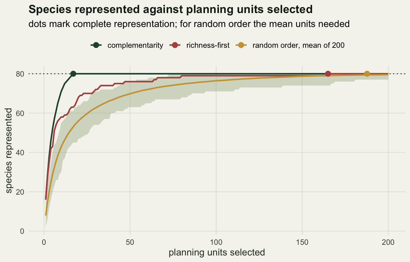

Figure 2: Species represented against planning units selected for the three rules, with the random baseline shown as the range across 200 replicates around its mean, and the points at which each rule reaches all 80 species.

The dot on the random line needs a word of care. It sits at the mean number of units needed for completeness, 187.72, which is not the same as the point where the mean curve crosses 80: averaging curves and averaging thresholds are different operations, and the mean curve stays slightly below the line past that point.

What the rule is actually doing

The mechanism is visible in when each species first gets covered. Under complementarity, restricted species come in early because they are the ones a unit can add that nothing else can. Under richness-first they come in whenever the ranking happens to stumble on them.

fs_greedy <- first_step(ord_greedy, pa)
cat("mean unit of first representation, species in 10 units or fewer:",
    "complementarity", round(mean(fs_greedy[range_size <= 10]), 2),
    " richness-first", round(mean(fs_rich[range_size <= 10]), 2), "\n")

mean unit of first representation, species in 10 units or fewer: complementarity 8.28  richness-first 31.39 

cat("Spearman correlation, range size against unit of first representation:",
    "complementarity", round(cor(range_size, fs_greedy,
                                 method = "spearman"), 4),
    " richness-first", round(cor(range_size, fs_rich,
                                 method = "spearman"), 4), "\n")

Spearman correlation, range size against unit of first representation: complementarity -0.5634  richness-first -0.6078 

cat("marginal species gained, first five steps: complementarity",
    cur_greedy[1:5] - c(0, cur_greedy[1:4]), "\n")

marginal species gained, first five steps: complementarity 16 12 10 8 6 

cat("marginal species gained, first five steps: richness-first",
    cur_rich[1:5] - c(0, cur_rich[1:4]), "\n")

marginal species gained, first five steps: richness-first 16 11 8 7 1 

For the 18 species confined to 10 units or fewer, the mean unit at which they first appear is 8.28 under complementarity and 31.39 under richness-first. Both rules cover widespread species early, which is why the Spearman correlation between range size and first representation is negative under both, -0.5634 and -0.6078; the difference is the scale on which the tail plays out.

The marginal gains are worth reading side by side. Both rules take the same first unit and gain 16 species. From the second step they diverge: complementarity gains 12, 10, 8, 6, while richness-first gains 11, 8, 7, 1. By its fifth pick the richness ranking is buying almost nothing, because it has picked four units from the same patch.

mech_df <- rbind(
  data.frame(range_size = range_size, step = fs_greedy,
             rule = "complementarity"),
  data.frame(range_size = range_size, step = fs_rich,
             rule = "richness-first"))
mech_df$rule <- factor(mech_df$rule,
                       levels = c("complementarity", "richness-first"))

ggplot(mech_df, aes(range_size, step, colour = rule)) +
  geom_point(size = 2, alpha = 0.8) +
  scale_x_log10() +
  scale_y_log10() +
  scale_colour_manual(values = c(te_pal$forest, te_pal$clay), name = NULL) +
  labs(title = "Restricted species wait longest under a richness ranking",
       subtitle = "each point is one species; lower is covered sooner",
       x = "range size, planning units occupied (log scale)",
       y = "unit of first representation (log scale)") +
  theme_te() +
  theme(legend.position = "top")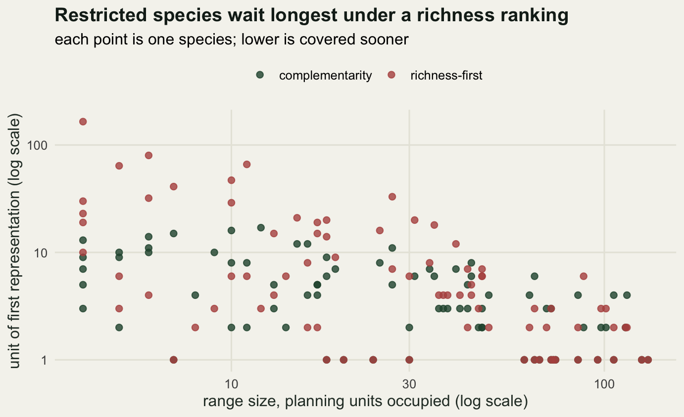

Figure 3: Range size against the unit at which each species is first represented, under richness-first and under greedy complementarity, both axes on a log scale.

What representation does not mean

Three limits belong on the same page as the 89.7 percent saving, because the number is only as meaningful as the target behind it.

Representation is not persistence. One recorded occurrence inside a selected unit says nothing about whether the population there is viable, connected to anything, or large enough to survive a bad decade. A target of one occurrence per species is an accounting convention that makes the mathematics tractable and the politics easier; it is not an ecological statement. Real planning sets larger targets, often a share of each species range, and the arithmetic above changes when it does.

Greedy is not optimal. The greedy rule is a heuristic: it takes the best step now and cannot undo it, and there exist sets smaller than 17 units that represent all 80 species here. The gap is usually small, but it is real, and no claim of optimality should be attached to any of these numbers. Measuring that gap against an exact solution is a separate exercise.

The species data is a model too. The presence-absence matrix here is exact by construction, which no real dataset is. False absences move priorities directly, because a rule that rewards a unit for holding the last unrepresented species is a rule that can be misled by a single missing record. That sensitivity is measurable, and it is the kind of thing worth measuring before a map is handed to anyone.

Where this goes next

Complementarity fixes the counting problem but ignores everything else a planner cares about. Units are not equally expensive, and a rule that spends the whole budget on the two most valuable parcels in the region is not useful however efficient it looks in species per unit. The next tutorial adds cost, replaces species per unit with species per unit of money, and measures how much more biodiversity the same budget buys once price is in the rule.

References

Kirkpatrick JB 1983 Biological Conservation 25(2):127-134 (10.1016/0006-3207(83)90056-3)

Vane-Wright RI, Humphries CJ, Williams PH 1991 Biological Conservation 55(3):235-254 (10.1016/0006-3207(91)90030-D)

Pressey RL, Humphries CJ, Margules CR, Vane-Wright RI, Williams PH 1993 Trends in Ecology and Evolution 8(4):124-128 (10.1016/0169-5347(93)90023-I)

Csuti B et al 1997 Biological Conservation 80(1):83-97 (10.1016/S0006-3207(96)00068-7)

Margules CR, Pressey RL 2000 Nature 405(6783):243-253 (10.1038/35012251)

Related tutorials

• Conservation costs and return on investment
• Compactness in reserve design
• Checking a conservation prioritisation
• Metapopulation capacity