library(ggplot2)

te_pal <- list(forest = "#275139", green = "#2f8f63", sage = "#93a87f",
               clay = "#b5534e", gold = "#cda23f", line = "#dad9ca",
               ink = "#16241d", paper = "#f5f4ee")

theme_te <- function() {
  theme_minimal(base_size = 12) +
    theme(panel.grid.minor = element_blank(),
          panel.grid.major = element_line(colour = "#e7e6dc"),
          plot.background = element_rect(fill = "#f5f4ee", colour = NA),
          panel.background = element_rect(fill = "#f5f4ee", colour = NA),
          plot.title = element_text(face = "bold", colour = te_pal$ink),
          axis.title = element_text(colour = "#2c3a31"))
}Checking a conservation prioritisation
R
conservation planning
model diagnostics
ecology tutorial
ggplot2
Four checks for a reserve selection plan in R: the gap between greedy and the exact optimum, run to run spread, data error, and how the target decides.
The three tutorials before this one built a prioritisation: greedy complementarity, cost as the budget, and a boundary length penalty solved by annealing. Each of them ends with a map of selected planning units, and a map of selected planning units is the most persuasive object in conservation science. It is also the output that hides the most.
This tutorial asks four questions of such a map, on simulated regions where the truth is available: how far from optimal is the heuristic, how much does the answer change between runs, what does an error in the input do to it, and how much of the answer was decided by the target rather than by the algorithm.
Check 1: how far from optimal is greedy?
Minimum set selection is NP-hard, so every real prioritisation uses a heuristic and nobody knows the size of the optimum. On instances small enough to enumerate, both numbers are available. Two functions: greedy complementarity, which repeatedly takes the unit covering the most species not yet covered, and an exact solver that encodes each unit’s species as a bit pattern and tests subsets in order of increasing size.
greedy_set <- function(pa) {
  need <- rep(TRUE, nrow(pa))
  picked <- integer(0)
  gains <- integer(0)
  while (any(need)) {
    gain <- colSums(pa[need, , drop = FALSE])
    gain[picked] <- -1L
    best <- which.max(gain)
    picked <- c(picked, best)
    gains <- c(gains, gain[best])
    need <- need & !pa[, best]
  }
  list(units = picked, gains = gains)
}

exact_set <- function(pa) {
  n_sp <- nrow(pa)
  n_u <- ncol(pa)
  masks <- as.integer(apply(pa, 2,
                            function(v) sum(as.integer(2^(which(v) - 1)))))
  full <- as.integer(2^n_sp - 1)
  for (k in seq_len(n_u)) {
    cmb <- combn(n_u, k)
    acc <- masks[cmb[1, ]]
    if (k > 1) for (r in 2:k) acc <- bitwOr(acc, masks[cmb[r, ]])
    hit <- which(acc == full)
    if (length(hit) > 0) {
      return(list(size = k, optima = cmb[, hit, drop = FALSE]))
    }
  }
  NULL
}

jaccard <- function(a, b) length(intersect(a, b)) / length(union(a, b))
The bit trick is what makes the exact solver usable in R. Each unit becomes one integer whose set bits are the species it holds, and bitwOr is vectorised, so all subsets of a given size are tested in a few vector operations rather than in a loop.
n_small <- 200
set.seed(4801)
insts <- vector("list", n_small)
for (i in seq_len(n_small)) {
  pa <- matrix(FALSE, 16, 14)
  rs <- sample(1:5, 16, replace = TRUE, prob = c(0.22, 0.30, 0.24, 0.14, 0.10))
  for (j in seq_len(16)) pa[j, sample(14, rs[j])] <- TRUE
  insts[[i]] <- pa
}

cmp <- data.frame(greedy = integer(n_small), exact = integer(n_small),
                  overlap = numeric(n_small))
for (i in seq_len(n_small)) {
  g <- greedy_set(insts[[i]])
  e <- exact_set(insts[[i]])
  cmp$greedy[i] <- length(g$units)
  cmp$exact[i] <- e$size
  cmp$overlap[i] <- max(apply(e$optima, 2, function(o) jaccard(g$units, o)))
}
cmp$excess <- cmp$greedy - cmp$exact

cat("instances tested:", n_small, " planning units each:", ncol(insts[[1]]),
    " species each:", nrow(insts[[1]]), "\n")
instances tested: 200 planning units each: 14 species each: 16 cat("instances where greedy is optimal:", round(mean(cmp$excess == 0), 4),
" as a percentage:", round(100 * mean(cmp$excess == 0), 2), "\n")instances where greedy is optimal: 0.78 as a percentage: 78 cat("mean excess:", round(mean(cmp$excess), 4), " worst excess:",
max(cmp$excess), " mean exact size:", round(mean(cmp$exact), 3), "\n")mean excess: 0.235 worst excess: 2 mean exact size: 5.855 cat("mean excess as a share of the optimum:",
round(mean(cmp$excess) / mean(cmp$exact), 4), " as a percentage:",
round(100 * mean(cmp$excess) / mean(cmp$exact), 2), "\n")mean excess as a share of the optimum: 0.0401 as a percentage: 4.01 cat("mean best overlap between the greedy set and an optimal set:",
round(mean(cmp$overlap), 4), "\n")mean best overlap between the greedy set and an optimal set: 0.9306 print(table(excess = cmp$excess))excess
0 1 2
156 41 3 cat("subsets to enumerate at 14 units:", 2^14,
" at 400 units: 10 to the power", round(400 * log10(2), 1), "\n")subsets to enumerate at 14 units: 16384 at 400 units: 10 to the power 120.4 Greedy finds an optimal set in 78 per cent of the 200 instances, costs 0.235 extra units on average against a mean optimum of 5.855, and in these 200 instances never needs more than two extra. In proportional terms it wastes 4.01 per cent of the reserve, and the units it picks overlap a genuinely optimal set at 0.9306. The instances where it loses are worth reading rather than counting, and the instance below shows the shape one such failure takes.
worst <- which(cmp$excess > 0 & cmp$exact == min(cmp$exact[cmp$excess > 0]))[1]
pa_w <- insts[[worst]]
dimnames(pa_w) <- list(paste0("sp", sprintf("%02d", 1:16)),
                       paste0("u", sprintf("%02d", 1:14)))
print(pa_w * 1L)
u01 u02 u03 u04 u05 u06 u07 u08 u09 u10 u11 u12 u13 u14
sp01 0 0 0 0 1 0 0 0 0 0 0 0 0 1
sp02 0 0 0 1 0 0 0 1 0 0 0 0 0 0
sp03 0 1 0 0 1 0 0 0 0 1 0 1 0 0
sp04 0 0 0 0 0 0 1 0 0 0 0 1 1 0
sp05 0 1 1 0 0 0 0 0 0 0 0 0 0 0
sp06 1 0 0 0 0 1 1 0 0 0 0 0 0 0
sp07 0 0 0 1 1 0 0 1 0 0 0 0 1 0
sp08 0 0 0 0 0 0 0 1 0 0 0 0 0 0
sp09 0 0 1 0 1 0 0 0 0 0 1 0 0 1
sp10 0 0 0 1 0 1 0 1 0 0 0 0 0 0
sp11 0 0 0 0 0 0 0 0 0 0 0 0 0 1
sp12 0 0 0 1 0 0 1 0 0 0 0 1 0 0
sp13 0 0 0 1 0 0 1 0 1 0 0 0 0 0
sp14 0 0 0 0 1 0 1 0 0 0 1 0 0 1
sp15 0 0 1 0 0 1 0 0 0 1 1 0 0 1
sp16 0 0 0 0 0 1 0 0 1 1 0 1 0 1gw <- greedy_set(pa_w)
ew <- exact_set(pa_w)
cat("greedy picks in order:", paste(colnames(pa_w)[gw$units], collapse = " "),
" new species at each pick:", paste(gw$gains, collapse = " "), "\n")greedy picks in order: u14 u04 u02 u07 u08 new species at each pick: 6 5 2 2 1 cat("optimal set of size", ew$size, ":",
paste(colnames(pa_w)[ew$optima[, 1]], collapse = " "),
" number of optimal sets:", ncol(ew$optima), "\n")optimal set of size 4 : u02 u07 u08 u14 number of optimal sets: 1 cat("units in the greedy set but not in the optimum:",
paste(setdiff(colnames(pa_w)[gw$units], colnames(pa_w)[ew$optima[, 1]]),
collapse = " "), "\n")units in the greedy set but not in the optimum: u04 forced <- which(colSums(pa_w[rowSums(pa_w) == 1, , drop = FALSE]) > 0)
cat("units holding a species found nowhere else:",
paste(colnames(pa_w)[forced], collapse = " "),
" greedy reached them at step:",
paste(match(forced, gw$units), collapse = " "), "\n")units holding a species found nowhere else: u08 u14 greedy reached them at step: 5 1 Greedy takes u14, u04, u02, u07, u08, gaining 6, 5, 2, 2 and 1 new species. The unique optimum is u02, u07, u08, u14: exactly the greedy set with u04 removed. The unit that looked second best on the day it was chosen turned out to be entirely redundant.
The reason is on the last printed line. Two units, u08 and u14, each hold a species that occurs nowhere else, so both are in every feasible solution before any algorithm starts. Greedy found u14 first because it was also the richest unit, but it did not reach u08 until step five, and u08 already supplied three of the five species that had made u04 attractive. Greedy is myopic in a specific way: it cannot use the fact that some units are compulsory.
exc_df <- as.data.frame(table(excess = cmp$excess))
exc_df$excess <- as.integer(as.character(exc_df$excess))
exc_df$label <- ifelse(exc_df$excess == 0, "optimal",
                       ifelse(exc_df$excess == 1, "1 extra unit",
                              paste(exc_df$excess, "extra units")))
exc_df$label <- factor(exc_df$label, levels = exc_df$label[order(exc_df$excess)])

ggplot(exc_df, aes(label, Freq)) +
  geom_col(fill = te_pal$forest, width = 0.6) +
  geom_text(aes(label = Freq), vjust = -0.4, colour = te_pal$ink, size = 4) +
  scale_y_continuous(limits = c(0, 178)) +
  labs(title = "Greedy is usually optimal, and sometimes is not",
       subtitle = "200 instances of 14 planning units and 16 species, solved exactly",
       x = "extra units in the greedy set", y = "instances") +
  theme_te()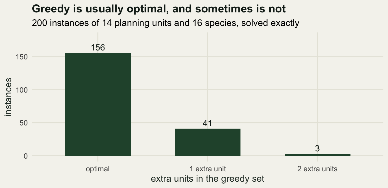
None of this generalises to a real region, and the last printed line says why. Enumerating 14 units means testing 16384 subsets; enumerating 400 units means testing about 10 to the power 120.4, which is not a computation, it is a number. A real analysis therefore cannot report a gap to the optimum. What it can report is a bound: the value of a linear programming relaxation, or the best objective from a very long annealing run used as a reference. “Greedy is close to optimal on small random instances” is a statement about small random instances, and quoting it as reassurance about a 400 unit plan is a category error.
Check 2: one map is not the answer
Move to a size where the exact answer is gone: a 20 by 20 grid of planning units, 60 species with clumped ranges, and a smoothly varying cost surface. Eight of the species occur on a single unit, which is the pattern that carries most of the signal in a real prioritisation.
smooth_field <- function(n, passes, seed) {
  set.seed(seed)
  z <- matrix(runif(n * n), n, n)
  for (p in seq_len(passes)) {
    pad <- rbind(z[1, ], z, z[n, ])
    pad <- cbind(pad[, 1], pad, pad[, n])
    z <- (pad[1:n, 2:(n + 1)] + pad[3:(n + 2), 2:(n + 1)] +
            pad[2:(n + 1), 1:n] + pad[2:(n + 1), 3:(n + 2)] +
            4 * pad[2:(n + 1), 2:(n + 1)]) / 8
  }
  (z - min(z)) / (max(z) - min(z))
}

gside <- 20
n_u <- gside * gside
n_sp <- 60
ux <- rep(seq_len(gside), each = gside)
uy <- rep(seq_len(gside), times = gside)
cost_u <- round(20 * exp(1.2 * as.vector(smooth_field(gside, 5, seed = 4812))), 1)

set.seed(4811)
radii <- c(rep(0, 8), exp(runif(n_sp - 8, log(1.15), log(4.6))))
occ <- matrix(FALSE, n_sp, n_u)
for (j in seq_len(n_sp)) {
  cx <- runif(1, 1, gside)
  cy <- runif(1, 1, gside)
  dd <- sqrt((ux - cx)^2 + (uy - cy)^2)
  inr <- which(dd <= radii[j])
  if (length(inr) == 0) inr <- which.min(dd)
  keep <- inr[runif(length(inr)) < 0.85]
  if (length(keep) == 0) keep <- inr[which.min(dd[inr])]
  occ[j, keep] <- TRUE
}
rng_sp <- rowSums(occ)

cat("range sizes: median", median(rng_sp), " smallest", min(rng_sp),
    " largest", max(rng_sp), " species on one unit only:", sum(rng_sp == 1), "\n")
range sizes: median 12.5 smallest 1 largest 54 species on one unit only: 8 cat("units holding at least one species:", sum(colSums(occ) > 0), "of", n_u, "\n")units holding at least one species: 352 of 400 cat("cost per unit: min", min(cost_u), " median", median(cost_u),
" max", max(cost_u), "\n")cost per unit: min 20 median 33.2 max 66.4 The optimiser is a compact version of the annealer from the compactness tutorial: one unit flipped at a time, the objective change computed incrementally from that unit’s cost, its selected neighbours and its species, and a geometric cooling schedule. The boundary term uses the identity that the perimeter of a set of grid cells is four times its size minus the number of adjacent selected pairs counted once each way, which turns a boundary calculation into a neighbour count.
nbrs <- vector("list", n_u)
for (i in seq_len(n_u)) {
  nn <- integer(0)
  if (ux[i] > 1) nn <- c(nn, i - gside)
  if (ux[i] < gside) nn <- c(nn, i + gside)
  if (uy[i] > 1) nn <- c(nn, i - 1L)
  if (uy[i] < gside) nn <- c(nn, i + 1L)
  nbrs[[i]] <- nn
}
spp_of <- lapply(seq_len(n_u), function(u) which(occ[, u]))

objective <- function(state, blm, pen) {
  pairs <- 0
  for (u in which(state)) pairs <- pairs + sum(state[nbrs[[u]]])
  sum(cost_u[state]) + blm * (4 * sum(state) - pairs) +
    pen * sum(rowSums(occ[, state, drop = FALSE]) == 0)
}

anneal <- function(seed, blm = 4, pen = 400, iters = 30000, t0 = 60, t1 = 0.05) {
  set.seed(seed)
  state <- runif(n_u) < 0.1
  cnt <- as.integer(rowSums(occ[, state, drop = FALSE]))
  temps <- t0 * (t1 / t0)^(seq_len(iters) / iters)
  which_u <- sample.int(n_u, iters, replace = TRUE)
  coin <- runif(iters)
  for (it in seq_len(iters)) {
    u <- which_u[it]
    sel <- state[u]
    sp <- spp_of[[u]]
    k <- sum(state[nbrs[[u]]])
    if (!sel) {
      d <- cost_u[u] + blm * (4 - 2 * k)
      if (length(sp)) d <- d - pen * sum(cnt[sp] == 0L)
    } else {
      d <- -cost_u[u] - blm * (4 - 2 * k)
      if (length(sp)) d <- d + pen * sum(cnt[sp] == 1L)
    }
    if (d <= 0 || coin[it] < exp(-d / temps[it])) {
      state[u] <- !sel
      if (length(sp)) cnt[sp] <- cnt[sp] + if (sel) -1L else 1L
    }
  }
  state
}
Now run it forty times from forty random starts, at one fixed boundary length modifier, and look at what varies.
n_run <- 40
runs <- lapply(seq_len(n_run), function(r) anneal(seed = 5100 + r))
objs <- vapply(runs, objective, 0, blm = 4, pen = 400)

cat("every run meets every target:",
    all(vapply(runs, function(s) all(rowSums(occ[, s, drop = FALSE]) > 0), TRUE)),
    "\n")
every run meets every target: TRUE cat("final objective: best", round(min(objs), 1), " mean", round(mean(objs), 1),
" worst", round(max(objs), 1), " worst over best",
round(max(objs) / min(objs), 4), "\n")final objective: best 1226.7 mean 1315.5 worst 1447.6 worst over best 1.1801 cat("units selected: min", min(vapply(runs, sum, 0L)),
" max", max(vapply(runs, sum, 0L)), "\n")units selected: min 26 max 31 pairs_j <- numeric(0)
for (a in seq_len(n_run - 1)) for (b in (a + 1):n_run) {
pairs_j <- c(pairs_j, sum(runs[[a]] & runs[[b]]) / sum(runs[[a]] | runs[[b]]))
}
cat("runs:", n_run, " grid side:", gside, " planning units:", n_u,
" species:", n_sp, "\n")runs: 40 grid side: 20 planning units: 400 species: 60 cat("mean pairwise Jaccard overlap between the plans:",
round(mean(pairs_j), 4), " range", round(min(pairs_j), 4), "to",
round(max(pairs_j), 4), "\n")mean pairwise Jaccard overlap between the plans: 0.2733 range 0.16 to 0.4857 cat("the same two overlaps as percentages: mean",
round(100 * mean(pairs_j), 2), " most similar pair",
round(100 * max(pairs_j), 2), "\n")the same two overlaps as percentages: mean 27.33 most similar pair 48.57 sel_freq <- rowMeans(do.call(cbind, lapply(runs, as.numeric)))
cat("units selected in more than 90 percent of runs:", sum(sel_freq > 0.9),
" in fewer than 10 percent:", sum(sel_freq < 0.1), "\n")units selected in more than 90 percent of runs: 8 in fewer than 10 percent: 309 Every run meets every target and selects between 26 and 31 units, so all forty are plausible plans. The objective ranges from 1226.7 to 1447.6, the worst run being 1.1801 times the best, which is a spread a single run cannot tell you about. The number that matters is the last pair. Two of the forty plans, chosen at random, share only 27.33 per cent of the units either one selects, and the most similar pair in the set shares 48.57 per cent. A single annealing run is one draw from a wide distribution of near equivalent plans, and printing it as “the priority areas” is a claim the optimiser does not support.
Selection frequency is the output that does survive. Eight units are selected in more than 90 per cent of runs and 309 of the 400 in fewer than 10 per cent, so the map holds a stable core and a large indifferent remainder.
endemic_u <- colSums(occ[rng_sp == 1, , drop = FALSE])
rarity_w <- colSums(occ / rng_sp)
has_sp <- colSums(occ) > 0

cat("units holding a species found nowhere else:", sum(endemic_u > 0),
    " their selection frequencies:",
    paste(round(sel_freq[endemic_u > 0], 3), collapse = " "), "\n")
units holding a species found nowhere else: 8 their selection frequencies: 1 1 1 1 1 1 1 1 cat("Spearman, selection frequency against rarity-weighted richness:",
round(cor(sel_freq[has_sp], rarity_w[has_sp], method = "spearman"), 4),
" against plain richness:",
round(cor(sel_freq[has_sp], colSums(occ)[has_sp], method = "spearman"), 4),
"\n")Spearman, selection frequency against rarity-weighted richness: 0.6288 against plain richness: 0.3978 The stable core is exactly the compulsory part of the problem. All eight units holding a species found nowhere else have a selection frequency of 1, which is the irreplaceability idea of Pressey and colleagues arriving from the other direction: a unit is irreplaceable when no solution can omit it, and a stochastic optimiser discovers that without being told.
Beyond those eight, the ranking by selection frequency tracks rarity-weighted richness (the sum over the species present of one over each species’ range size) at a Spearman correlation of 0.6288, against 0.3978 for plain species richness. Selecting the richest units is the mistake the complementarity tutorial started with, and the pair of correlations puts a number on it. Neither cheap index reproduces the annealer’s priorities, because cost is in the objective as well.
map_df <- rbind(
  data.frame(x = ux, y = uy, freq = as.numeric(runs[[1]]),
             panel = "one run, one map"),
  data.frame(x = ux, y = uy, freq = sel_freq,
             panel = "40 runs, selection frequency"))
map_df$panel <- factor(map_df$panel,
                       levels = c("one run, one map",
                                  "40 runs, selection frequency"))
mark <- data.frame(
  x = rep(ux[endemic_u > 0], 2), y = rep(uy[endemic_u > 0], 2),
  panel = factor(rep(levels(map_df$panel), each = sum(endemic_u > 0)),
                 levels = levels(map_df$panel)))

ggplot(map_df, aes(x, y)) +
  geom_raster(aes(fill = freq)) +
  geom_point(data = mark, colour = te_pal$clay, size = 2, shape = 1,
             stroke = 1.1) +
  facet_wrap(~panel) +
  coord_equal() +
  scale_fill_gradient(low = te_pal$paper, high = te_pal$forest,
                      name = "frequency", limits = c(0, 1)) +
  labs(title = "One plan is one draw from many",
       subtitle = "circles: units holding a species found nowhere else",
       x = NULL, y = NULL) +
  theme_te() +
  theme(axis.text = element_blank(), panel.grid = element_blank())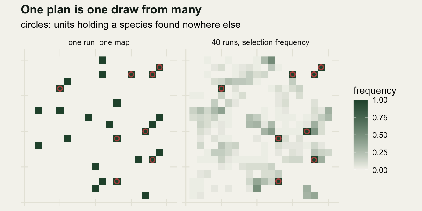
Check 3: what does an error in the data do to the plan?
Two errors, both measured the same way. First, false absences: keep each occurrence record with probability 0.9, 0.7 or 0.5, and re-select. Second, cost error: multiply every unit cost by lognormal noise and re-select. For each perturbed plan, measure the overlap with the plan built on the complete data, and the representation the perturbed plan actually achieves when scored against the true species data.
The selection here is a cost-effective greedy pass rather than the annealer, so that the replicate re-runs stay cheap. It takes the unit with the best ratio of unmet target contribution to cost.
greedy_plan <- function(pa, cost_v, target, top = 1L) {
  covered <- integer(nrow(pa))
  picked <- integer(0)
  repeat {
    short <- target > covered
    if (!any(short)) break
    gain <- colSums(pa[short, , drop = FALSE])
    gain[picked] <- 0L
    if (all(gain == 0L)) break
    score <- gain / cost_v
    if (top > 1L) {
      pool <- order(score, decreasing = TRUE)[seq_len(min(top, sum(score > 0)))]
      best <- if (length(pool) == 1L) pool else sample(pool, 1)
    } else {
      best <- which.max(score)
    }
    picked <- c(picked, best)
    covered <- covered + as.integer(pa[, best])
  }
  sort(picked)
}

base_plan <- greedy_plan(occ, cost_u, rep(1L, n_sp))
cat("baseline plan: units", length(base_plan), " cost",
    round(sum(cost_u[base_plan]), 1), " species represented",
    round(mean(rowSums(occ[, base_plan, drop = FALSE]) > 0), 4), "\n")
baseline plan: units 25 cost 784.3 species represented 1 n_pert <- 30
set.seed(4821)
pert <- NULL
van_rng <- list()
for (p_det in c(0.9, 0.7, 0.5)) {
ov <- numeric(n_pert)
rep_true <- numeric(n_pert)
lost <- numeric(n_pert)
ranges_lost <- numeric(0)
for (r in seq_len(n_pert)) {
obs <- occ & matrix(runif(n_sp * n_u) < p_det, n_sp, n_u)
seen <- rowSums(obs) > 0
pl <- greedy_plan(obs[seen, , drop = FALSE], cost_u, rep(1L, sum(seen)))
ov[r] <- jaccard(pl, base_plan)
rep_true[r] <- mean(rowSums(occ[, pl, drop = FALSE]) > 0)
lost[r] <- sum(!seen)
ranges_lost <- c(ranges_lost, rng_sp[!seen])
}
van_rng[[as.character(p_det)]] <- ranges_lost
pert <- rbind(pert, data.frame(
kind = "false absences", setting = p_det, input_err = round(1 - p_det, 3),
overlap = round(mean(ov), 4), represented = round(mean(rep_true), 4),
spp_lost = round(mean(lost), 2), cost_ratio = NA_real_))
}
for (sig in c(0.25, 0.5, 1)) {
ov <- numeric(n_pert)
rep_true <- numeric(n_pert)
cr <- numeric(n_pert)
err <- numeric(n_pert)
for (r in seq_len(n_pert)) {
noise <- exp(rnorm(n_u, 0, sig))
pl <- greedy_plan(occ, cost_u * noise, rep(1L, n_sp))
ov[r] <- jaccard(pl, base_plan)
rep_true[r] <- mean(rowSums(occ[, pl, drop = FALSE]) > 0)
cr[r] <- sum(cost_u[pl]) / sum(cost_u[base_plan])
err[r] <- median(abs(noise - 1))
}
pert <- rbind(pert, data.frame(
kind = "cost error", setting = sig, input_err = round(mean(err), 3),
overlap = round(mean(ov), 4), represented = round(mean(rep_true), 4),
spp_lost = NA_real_, cost_ratio = round(mean(cr), 4)))
}
print(pert, row.names = FALSE) kind setting input_err overlap represented spp_lost cost_ratio
false absences 0.90 0.100 0.6427 0.9822 1.07 NA
false absences 0.70 0.300 0.3993 0.9606 2.50 NA
false absences 0.50 0.500 0.2786 0.9183 5.40 NA
cost error 0.25 0.168 0.3921 1.0000 NA 1.1309
cost error 0.50 0.327 0.2970 1.0000 NA 1.2750
cost error 1.00 0.589 0.2441 1.0000 NA 1.4047cat("median range size of the species that vanished, by detection probability:",
paste(names(van_rng), vapply(van_rng, function(v) median(v), 0),
sep = ":", collapse = " "), " largest range lost:",
max(vapply(van_rng, function(v) max(v), 0)),
" median range in the whole set:", median(rng_sp), "\n")median range size of the species that vanished, by detection probability: 0.9:1 0.7:1 0.5:1 largest range lost: 7 median range in the whole set: 12.5 Start with the fairness of the comparison, because it is the part most sensitivity analyses skip. A detection probability and a lognormal spread are not on a common scale, and nothing makes them so. The input_err column is the closest available proxy: one minus detection for the records, and the median absolute relative cost change for the costs. On that axis a detection probability of 0.7 (0.300 of records deleted) sits next to a lognormal sigma of 0.5 (0.327 median cost change), so those two rows are the honest pairing, and it is an approximate one.
At that matched pair the cost error moves the plan slightly more: overlap 0.2970 against 0.3993 for the false absences. If the question is “will my map change”, cost error is the bigger threat, and at sigma of 1 the overlap falls to 0.2441 while the true cost of the chosen plan rises to 1.4047 times the baseline.
The represented column is the one that should end the argument. A plan built on gappy records covers every species it can see, and then represents only 0.9606 of the species that are really there at a detection of 0.7, and 0.9183 at a detection of 0.5. Cost error leaves representation at 1.0000 at every level, because the species data were never touched. The two failures are of different kinds: cost error rearranges the map, whereas false absences leave species unprotected while the reserve report states full coverage.
The last printed line says which species. The median range size of a species that disappears from the data is 1, against a median of 12.5 across all 60 species, and the species that vanish sit at the small-range end of that distribution. Records are lost precisely when a range is small, which is to say precisely when the species is the reason for the plan.
pert_long <- rbind(
  data.frame(kind = pert$kind, change = pert$input_err, value = pert$overlap,
             measure = "overlap with the true-data plan"),
  data.frame(kind = pert$kind, change = pert$input_err,
             value = pert$represented,
             measure = "species represented in the true data"))
pert_long$kind <- factor(pert_long$kind,
                         levels = c("false absences", "cost error"))

ggplot(pert_long, aes(change, value, colour = measure, shape = measure)) +
  geom_line(linewidth = 0.7) +
  geom_point(size = 2.6) +
  facet_wrap(~kind) +
  scale_colour_manual(values = c(te_pal$clay, te_pal$forest), name = NULL) +
  scale_shape_manual(values = c(16, 17), name = NULL) +
  coord_cartesian(ylim = c(0, 1.05)) +
  labs(title = "Two input errors, measured the same way",
       subtitle = paste("x axis: proportion of records deleted (left),",
                        "median absolute relative cost change (right)"),
       x = "size of the input error", y = "proportion") +
  theme_te() +
  theme(legend.position = "bottom")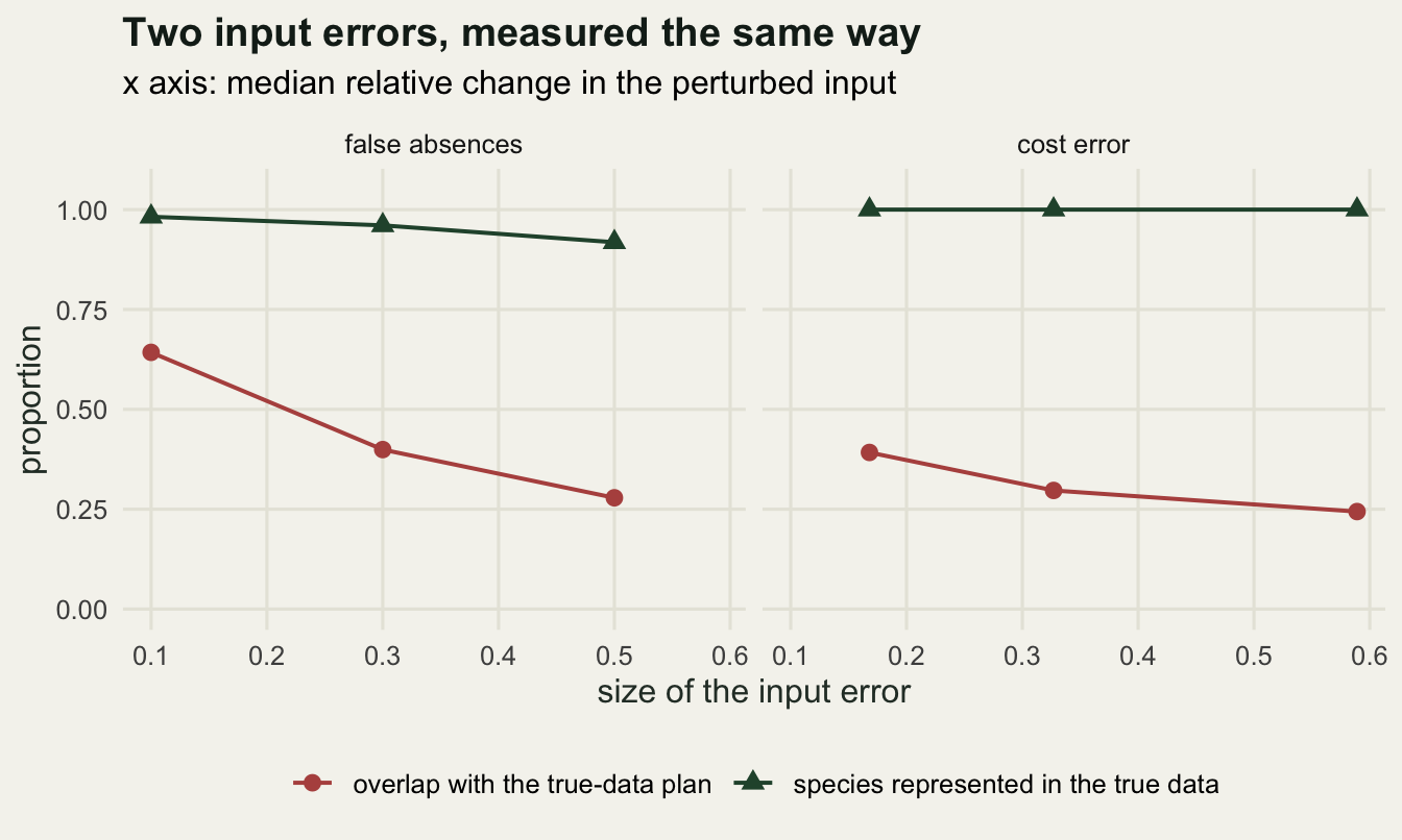
Check 4: the currency decides the ranking
Same species data, same costs, three targets. One occurrence per species is the textbook minimum set. Twenty per cent of each species’ range is the standard proportional target. The third is a range-size weighted target of the kind Rodrigues and Gaston discuss: restricted species get a high proportion of their range, widespread species a low one, interpolated on log range. The weighting is scaled so that it demands almost the same total number of occurrences as the flat 20 per cent rule, which keeps the comparison about emphasis rather than about stringency.
Priorities come from selection frequency again, this time over 40 randomised greedy runs that pick at random among the three best-scoring units at each step.
prop_target <- function(rng_v, lo = 4, hi = 64, p_lo = 0.5, p_hi = 0.04) {
  w <- (log(pmin(pmax(rng_v, lo), hi)) - log(lo)) / (log(hi) - log(lo))
  pmax(1L, ceiling((p_lo + w * (p_hi - p_lo)) * rng_v))
}

tg <- list(`one occurrence` = rep(1L, n_sp),
           `20 percent of range` = pmax(1L, ceiling(0.2 * rng_sp)),
           `rarity-weighted` = prop_target(rng_sp))
print(data.frame(scheme = names(tg),
                 occurrences_required = vapply(tg, function(v) sum(v), 0),
                 median_target = vapply(tg, function(v) median(v), 0),
                 largest_target = vapply(tg, function(v) max(v), 0)),
      row.names = FALSE)
scheme occurrences_required median_target largest_target
one occurrence 60 1 1
20 percent of range 208 3 11
rarity-weighted 219 4 5set.seed(4831)
freq_tg <- lapply(tg, function(target) {
hits <- integer(n_u)
for (r in seq_len(40)) {
pl <- greedy_plan(occ, cost_u, target, top = 3L)
hits[pl] <- hits[pl] + 1L
}
hits / 40
})
rank_cor <- function(a, b) {
round(cor(freq_tg[[a]], freq_tg[[b]], method = "spearman"), 4)
}
top20 <- lapply(freq_tg, function(f) order(f, rarity_w, decreasing = TRUE)[1:20])
shared <- function(a, b) length(intersect(top20[[a]], top20[[b]]))
nm <- names(tg)
n_top <- 20
cat("randomised greedy runs per scheme:", 40, " units ranked:", n_u,
" top set size:", n_top, "\n")randomised greedy runs per scheme: 40 units ranked: 400 top set size: 20 cat("units selected at least once:",
paste(vapply(freq_tg, function(f) sum(f > 0), 0), collapse = " "), "\n")units selected at least once: 67 106 125 tg_tab <- data.frame(
comparison = c(paste(nm[1], "vs", nm[2]), paste(nm[1], "vs", nm[3]),
paste(nm[2], "vs", nm[3])),
spearman = c(rank_cor(1, 2), rank_cor(1, 3), rank_cor(2, 3)),
shared_20 = c(shared(1, 2), shared(1, 3), shared(2, 3)))
tg_tab$jaccard_20 <- round(tg_tab$shared_20 / (40 - tg_tab$shared_20), 4)
print(tg_tab, row.names = FALSE) comparison spearman shared_20 jaccard_20
one occurrence vs 20 percent of range 0.6433 12 0.4286
one occurrence vs rarity-weighted 0.6876 13 0.4815
20 percent of range vs rarity-weighted 0.8006 11 0.3793The three schemes demand 60, 208 and 219 occurrences and touch 67, 106 and 125 of the 400 units at least once. Their unit rankings correlate at Spearman 0.6433, 0.6876 and 0.8006, and their top twenty units share 12, 13 and 11 members, which as a Jaccard overlap of the top twenty is 0.4286, 0.4815 and 0.3793.
Put that beside Check 1. There, swapping greedy for a proven optimum left the selected units overlapping at 0.9306 and cost 4.01 per cent in reserve size. Here, swapping a one-occurrence target for a proportional one drops the overlap of the top twenty to 0.4286. The target is not a technical setting; it is a value judgement about how much of each species is enough, made before any data are analysed, and it moves the answer roughly an order of magnitude further from agreement than the choice of algorithm did on those small instances. A prioritisation paper that reports its solver in detail and its target in half a sentence has documented the smaller decision.
tg_long <- do.call(rbind, lapply(seq_along(freq_tg), function(k) {
  data.frame(x = ux, y = uy, freq = freq_tg[[k]], scheme = nm[k],
             top = seq_len(n_u) %in% top20[[k]])
}))
tg_long$scheme <- factor(tg_long$scheme, levels = nm)

ggplot(tg_long, aes(x, y)) +
  geom_raster(aes(fill = freq)) +
  geom_point(data = subset(tg_long, top), colour = te_pal$clay, size = 1.4) +
  facet_wrap(~scheme) +
  coord_equal() +
  scale_fill_gradient(low = te_pal$paper, high = te_pal$forest,
                      name = "selection\nfrequency", limits = c(0, 1)) +
  labs(title = "The target moves the priorities",
       subtitle = "dots mark each scheme's top twenty units",
       x = NULL, y = NULL) +
  theme_te() +
  theme(axis.text = element_blank(), panel.grid = element_blank())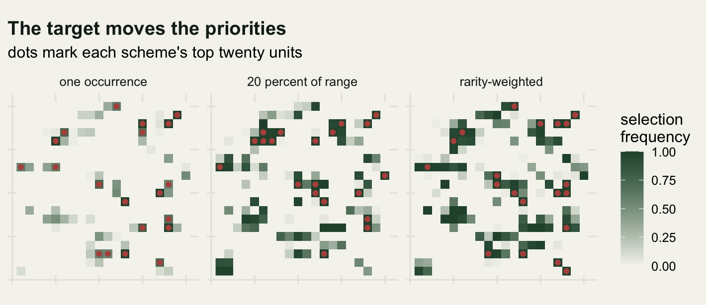
The honest limit
The four checks constrain a prioritisation. None of them validates it, and the gap is not a matter of degree.
Every quantity above comes from the same three inputs: a species by unit occurrence matrix, a cost vector, and a target. Nothing inside that triple can tell you whether an occurrence record means a population that will persist or a vagrant seen once, whether the cost vector is the cost that will really be paid, or whether a unit selected today will still hold its species in thirty years. Meir and colleagues showed that a plan built on a static snapshot can do worse than a simple opportunistic rule when land is lost while the analysis proceeds; Grantham and colleagues put a price on waiting for better data; Kujala and colleagues catalogue how input uncertainty propagates into the map. None of the three has an algorithmic answer.
So the two fixes are not better solvers. The first is data on persistence rather than on presence: repeat surveys that estimate detection, and some evidence that the populations are viable, because the species lost from a gappy data set had a median range of 1 unit, which is exactly the set the plan exists to protect. The second is a plan that is revisited on a schedule, with selection frequency rather than a single map as the standing output, so that the indifferent 309 units stay available for the next round instead of being written off by one annealing run that started from one particular random state.
Where to go next
That is the conservation planning cluster complete: complementarity, cost, compactness, and now the checks. The same four questions apply almost unchanged to a connectivity analysis, where the arbitrary input is a resistance value rather than a target, and the tutorial on checking a connectivity analysis works through them on simulated landscapes where the movement process is known.
References
Pressey RL, Johnson IR, Wilson PD 1994 Biodiversity and Conservation 3(3):242-262 (10.1007/BF00055941)
Rodrigues ASL, Gaston KJ 2002 Biological Conservation 107(1):123-129 (10.1016/S0006-3207(02)00042-3)
Meir E, Andelman S, Possingham HP 2004 Ecology Letters 7(8):615-622 (10.1111/j.1461-0248.2004.00624.x)
Grantham HS, Wilson KA, Moilanen A, Rebelo T, Possingham HP 2009 Ecology Letters 12(4):293-301 (10.1111/j.1461-0248.2009.01287.x)
Kujala H, Burgman MA, Moilanen A 2013 Conservation Letters 6(2):73-85 (10.1111/j.1755-263X.2012.00299.x)