library(ggplot2)

te_pal <- list(forest = "#275139", green = "#2f8f63", sage = "#93a87f",
               clay = "#b5534e", gold = "#cda23f", line = "#dad9ca",
               ink = "#16241d", paper = "#f5f4ee")

theme_te <- function() {
  theme_minimal(base_size = 12) +
    theme(panel.grid.minor = element_blank(),
          panel.grid.major = element_line(colour = "#e7e6dc"),
          plot.background = element_rect(fill = "#f5f4ee", colour = NA),
          panel.background = element_rect(fill = "#f5f4ee", colour = NA),
          plot.title = element_text(face = "bold", colour = te_pal$ink),
          axis.title = element_text(colour = "#2c3a31"))
}Conservation costs and return on investment
R
conservation planning
biodiversity
ecology tutorial
ggplot2
Reserve selection with a land price surface in R: three greedy rules under a fixed budget, and the gain from maximising species represented per pound spent.
The previous tutorial counted planning units. Every unit was treated as equally available, so “the smallest number of units that represents every species” was a reasonable objective, and greedy complementarity beat picking the richest units by a wide margin. Land does not behave that way. Within one region the price of a hectare can vary by two orders of magnitude, and the expensive ground is often the ground with the most species on it, because warm, fertile, low-lying land is both productive and valuable.
So the plan that represents the most species per unit selected is not the plan that represents the most species per pound spent. Naidoo and colleagues set out the case for putting money rather than area on the horizontal axis, and this tutorial measures it: a planning region with a price surface, three greedy rules against a fixed budget, and the value of accounting for price at a fixed budget, at a fixed representation target, and as a function of how strongly price tracks richness.
A region with a price tag
The generator lives in one function so that the last section can vary one argument and hold everything else fixed. Species ranges come from smoothed random fields, thresholded at a species-specific range size, and pushed towards one end of an environmental gradient so that richness is spatially clustered rather than uniform.
The price surface is built by mixing the richness surface with an independent smooth field, smoothing the mixture, and mapping its rank onto a price range spanning two orders of magnitude. The mixing weight is the dial: it sets how tightly price follows richness without touching the species data at all.
smooth_pass <- function(z, passes) {
  n <- nrow(z)
  for (p in seq_len(passes)) {
    pad <- rbind(z[1, ], z, z[n, ])
    pad <- cbind(pad[, 1], pad, pad[, n])
    z <- (pad[1:n, 2:(n + 1)] + pad[3:(n + 2), 2:(n + 1)] +
            pad[2:(n + 1), 1:n] + pad[2:(n + 1), 3:(n + 2)] +
            4 * pad[2:(n + 1), 2:(n + 1)]) / 8
  }
  z
}

smooth_field <- function(n, passes, seed) {
  set.seed(seed)
  z <- smooth_pass(matrix(runif(n * n), n, n), passes)
  (z - min(z)) / (max(z) - min(z))
}

zscore <- function(x) (x - mean(x)) / sd(x)

make_region <- function(n_side = 20, n_species = 80, price_link = 0.92,
                        bias = 0.3, med_size = 6, size_sd = 0.8, span = 100,
                        skew = 2.5, price_smooth = 2, seed = 5117) {
  n_units <- n_side * n_side
  gradient <- as.vector(smooth_field(n_side, 5, seed))
  unrelated <- as.vector(smooth_field(n_side, 5, seed + 1))
  set.seed(seed + 2)
  range_size <- pmax(2, pmin(150, round(rlnorm(n_species, log(med_size),
                                               size_sd))))
  pres <- matrix(FALSE, n_units, n_species)
  for (s in seq_len(n_species)) {
    field <- as.vector(smooth_field(n_side, 3, seed + 100 + s))
    pull <- zscore(field) + bias * zscore(gradient)
    pres[order(pull, decreasing = TRUE)[seq_len(range_size[s])], s] <- TRUE
  }
  rich <- rowSums(pres)
  mix <- price_link * zscore(rich) + sqrt(1 - price_link^2) * zscore(unrelated)
  latent <- as.vector(smooth_pass(matrix(mix, n_side, n_side), price_smooth))
  quant <- (rank(latent) - 0.5) / n_units
  price <- 3 * span^(quant^skew)
  list(n_side = n_side, pres = pres, price = price, rich = rich,
       range_size = range_size)
}
Two details in that code carry the argument. The quant^skew term makes the price distribution right-skewed: most of the region is cheap and a small part holds most of the value, which is how land markets look. And because quant is a rank, the set of prices is the same whatever the mixing weight; only which unit gets which price changes. That keeps the last experiment clean, because the total value of the region cannot drift between runs.
reg <- make_region()
pres <- reg$pres
price <- reg$price
total <- sum(price)
dear <- order(price, decreasing = TRUE)

cat("planning units:", nrow(pres), " species:", ncol(pres), "\n")
planning units: 400 species: 80 cat("range size, units occupied: min", min(reg$range_size),
" median", median(reg$range_size), " max", max(reg$range_size), "\n")range size, units occupied: min 2 median 6 max 62 cat("species per unit: min", min(reg$rich), " mean", round(mean(reg$rich), 2),
" max", max(reg$rich), "\n")species per unit: min 0 mean 1.68 max 18 cat("price: min", round(min(price), 2), " max", round(max(price), 2),
" ratio", round(max(price) / min(price), 1), "\n")price: min 3 max 295.72 ratio 98.6 cat("total land value:", round(total), "\n")total land value: 12839 cat("percent of total value in the most expensive 10 percent of units:",
round(100 * sum(price[dear[1:40]]) / total, 2), "\n")percent of total value in the most expensive 10 percent of units: 56.69 cat("units buyable for 15 percent of the total value, cheapest first:",
sum(cumsum(sort(price)) <= 0.15 * total), "\n")units buyable for 15 percent of the total value, cheapest first: 289 cat("Spearman correlation, price against species richness:",
round(cor(price, reg$rich, method = "spearman"), 4), "\n")Spearman correlation, price against species richness: 0.6865 cat("species confined to the most expensive quarter of the region:",
sum(apply(pres, 2, function(s) all(which(s) %in% dear[1:100]))), "\n")species confined to the most expensive quarter of the region: 14 The region holds 400 units and 80 species, with ranges from 2 to 62 units (median 6) and between 0 and 18 species per unit. Prices run from 3 to 295.72, a ratio of 98.6, and the realised rank correlation between price and richness is 0.6865. That is a strong association, at the upper end of what field studies report, and the last section covers the weaker cases.
Two numbers describe the market and they matter more than they look. The most expensive tenth of the region holds 56.69 per cent of its total value, and 289 of the 400 units can be bought for 15 per cent of that value if you buy from the bottom of the price list. Meanwhile 14 species occur nowhere except in the most expensive quarter of the region, so no amount of cheap land will represent them.
Three greedy rules under one budget
Each rule is the same loop with a different score. The cost-blind rule takes the unit that adds the most species not yet represented, which is the rule from the previous tutorial. The cost-only rule takes the cheapest remaining unit and ignores biodiversity completely. The benefit-cost rule takes the unit with the best ratio of new species to price.
The budget convention: at every step the rule chooses among the units it can still afford, and it stops when nothing affordable is left or when every species is represented. That is the charitable reading of a cost-blind plan, since it is never blocked outright by one unaffordable parcel.
greedy_plan <- function(pres, price, budget, rule) {
  covered <- rep(FALSE, ncol(pres))
  taken <- rep(FALSE, nrow(pres))
  spent <- 0
  sel <- integer(0)
  repeat {
    if (all(covered)) break
    afford <- !taken & price <= budget - spent + 1e-9
    if (!any(afford)) break
    gain <- rowSums(pres[, !covered, drop = FALSE])
    score <- if (rule == "benefit") gain else
      if (rule == "cheapest") -price else gain / price
    score[!afford] <- -Inf
    if (rule != "cheapest" && max(score) <= 0) break
    pick <- which.max(score)
    taken[pick] <- TRUE
    spent <- spent + price[pick]
    covered <- covered | pres[pick, ]
    sel <- c(sel, pick)
  }
  list(sel = sel, spent = spent, species = sum(covered))
}
rule_key <- c("benefit", "cheapest", "ratio")
rule_name <- c("new species per unit", "cheapest first",
"new species per pound")
budget <- 0.15 * total
plan15 <- lapply(rule_key, function(r) greedy_plan(pres, price, budget, r))
tab15 <- data.frame(
rule = rule_name,
units = sapply(plan15, function(p) length(p$sel)),
spent = round(sapply(plan15, function(p) p$spent)),
species = sapply(plan15, function(p) p$species),
mean_price = round(sapply(plan15, function(p) mean(price[p$sel])), 1),
mean_richness = round(sapply(plan15, function(p) mean(reg$rich[p$sel])), 2))
cat("budget, 15 percent of the total land value:", round(budget), "\n")budget, 15 percent of the total land value: 1926 print(tab15, row.names = FALSE) rule units spent species mean_price mean_richness
new species per unit 13 1926 67 148.1 6.92
cheapest first 289 1903 64 6.6 0.87
new species per pound 58 1745 80 30.1 2.47cat("percent of the region's area bought:",
round(100 * tab15$units / nrow(pres), 2), "\n")percent of the region's area bought: 3.25 72.25 14.5 cat("species ratio, benefit-cost rule over cost-blind rule:",
round(plan15[[3]]$species / plan15[[1]]$species, 4),
" extra species:", plan15[[3]]$species - plan15[[1]]$species, "\n")species ratio, benefit-cost rule over cost-blind rule: 1.194 extra species: 13 With 1926 to spend, the cost-blind rule buys 13 units at a mean price of 148.1 and represents 67 species. The benefit-cost rule buys 58 units at a mean price of 30.1, represents all 80, and does it for 1745, leaving part of the budget unspent. The ratio between the two is 1.194, so 13 extra species from the same budget and a smaller outlay, and the only thing that changed is that the second rule divided by price before ranking.
The cost-only rule is the instructive failure. It spends 1903 on 289 units, 72.25 per cent of the region’s area, and comes away with 64 species. The units it bought hold 0.87 species each on average against 6.92 for the cost-blind rule. Buying cheap land is not a conservation plan; it is a way of owning a lot of ground that nobody was competing for.
map_df <- data.frame(x = rep(seq_len(reg$n_side), each = reg$n_side),
                     y = rep(seq_len(reg$n_side), times = reg$n_side),
                     price = price)
panels <- c("cost-blind rule: new species per unit",
            "benefit-cost rule: new species per pound")
sel_df <- rbind(data.frame(map_df[plan15[[1]]$sel, c("x", "y")],
                           plan = panels[1]),
                data.frame(map_df[plan15[[3]]$sel, c("x", "y")],
                           plan = panels[2]))
sel_df$plan <- factor(sel_df$plan, levels = panels)
grid_df <- do.call(rbind, lapply(panels, function(p) data.frame(map_df,
                                                               plan = p)))
grid_df$plan <- factor(grid_df$plan, levels = panels)

ggplot(grid_df, aes(x, y)) +
  geom_raster(aes(fill = log10(price))) +
  geom_point(data = sel_df, shape = 21, size = 2.1, stroke = 0.5,
             colour = "white", fill = te_pal$clay) +
  facet_wrap(~plan) +
  coord_equal() +
  scale_fill_gradient(low = te_pal$paper, high = te_pal$forest, name = "price",
                      breaks = log10(c(5, 20, 80, 250)),
                      labels = c(5, 20, 80, 250)) +
  labs(title = "One budget, two reserve networks",
       subtitle = "circles: units bought with 15 percent of the total land value",
       x = NULL, y = NULL) +
  theme_te() +
  theme(axis.text = element_blank(), panel.grid = element_blank())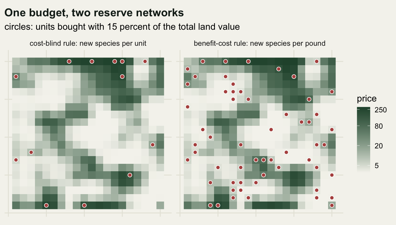
The mirror question: what does full representation cost?
A fixed budget is one of the two shapes a real plan takes. The other is a fixed target: every species has to be in, and the question is the bill. Running each rule with no budget ceiling answers it.
plan_full <- lapply(rule_key, function(r) greedy_plan(pres, price, Inf, r))
tabf <- data.frame(
  rule = rule_name,
  units = sapply(plan_full, function(p) length(p$sel)),
  spent = round(sapply(plan_full, function(p) p$spent)),
  percent_of_value = round(100 * sapply(plan_full,
                                        function(p) p$spent) / total, 2))
print(tabf, row.names = FALSE)
rule units spent percent_of_value
new species per unit 24 2929 22.81
cheapest first 394 11185 87.12
new species per pound 58 1745 13.59cat("cost of full representation, cost-blind over benefit-cost:",
round(plan_full[[1]]$spent / plan_full[[3]]$spent, 4),
" cheapest first over benefit-cost:",
round(plan_full[[2]]$spent / plan_full[[3]]$spent, 4), "\n")cost of full representation, cost-blind over benefit-cost: 1.6789 cheapest first over benefit-cost: 6.4109 The cost-blind rule reaches all 80 species with only 24 units, which is the result the previous tutorial was built to show, and it pays 2929, or 22.81 per cent of the region’s value. The benefit-cost rule needs 58 units, more than twice as many, and pays 1745, or 13.59 per cent. Counting units, the cost-blind plan wins comfortably. Counting money, it costs 1.6789 times as much for exactly the same representation.
Cost-only selection is worse than either by a long way: 394 units and 87.12 per cent of the region’s value, 6.4109 times the efficient plan, because the last species it needs happen to sit on the land it has been avoiding all along. Ando and colleagues reported the same asymmetry for United States counties in 1998, and it is the finding that started this literature.
The two framings give different-looking numbers from one set of facts, and both are worth reporting. A fixed budget makes the gain look modest, a species ratio of 1.194. A fixed target makes it look large, a cost factor of 1.6789. Neither is wrong: the first is bounded above by the number of species in the region and the second is not bounded at all, which is why the return-on-investment formulation of Murdoch and colleagues prefers the second.
The efficiency curve
One budget is a single slice through a curve. Recomputing each rule across the whole range of budgets shows where the rules separate and where they stop mattering.
fracs <- seq(0.025, 0.6, by = 0.025)
curve_df <- do.call(rbind, lapply(seq_along(rule_key), function(i) {
  data.frame(percent = round(100 * fracs, 3), rule = rule_name[i],
             species = sapply(fracs, function(f)
               greedy_plan(pres, price, f * total, rule_key[i])$species))
}))
curve_df$rule <- factor(curve_df$rule, levels = rule_name)

cat("budget range covered, percent of total value:",
    min(curve_df$percent), "to", max(curve_df$percent), "\n")
budget range covered, percent of total value: 2.5 to 60 key_rows <- curve_df[curve_df$percent %in% c(5, 15, 40), ]
print(key_rows[order(key_rows$percent), ], row.names = FALSE) percent rule species
5 new species per unit 42
5 cheapest first 46
5 new species per pound 71
15 new species per unit 67
15 cheapest first 64
15 new species per pound 80
40 new species per unit 80
40 cheapest first 72
40 new species per pound 80blind <- curve_df[curve_df$rule == rule_name[1], ]
for (i in seq_along(rule_name)) {
s <- curve_df$species[curve_df$rule == rule_name[i]]
cat(rule_name[i], "| increasing throughout:", all(diff(s) >= 0), "\n")
}new species per unit | increasing throughout: FALSE
cheapest first | increasing throughout: TRUE
new species per pound | increasing throughout: TRUE cat("cost-blind rule at 7.5 and at 10 percent of the total value:",
blind$species[blind$percent == 7.5], blind$species[blind$percent == 10],
"\n")cost-blind rule at 7.5 and at 10 percent of the total value: 57 54 At 5 per cent of the region’s value the three rules give 42, 46 and 71 species: the benefit-cost rule already has nearly everything while the other two have about half. At 15 per cent they give 67, 64 and 80. At 40 per cent the two complementarity rules have converged on all 80 and cost-only selection has still only reached 72, because the units holding the species it lacks are the ones it buys last.
On this run the cost-blind curve is not even increasing throughout. It reaches 57 species at 7.5 per cent of the total value and 54 at 10 per cent. That is not a bug: a larger budget lets the rule afford an expensive high-benefit unit early, and buying it consumes money that would otherwise have bought several cheaper units later. A ranking that ignores price can be unstable with respect to the budget as well as inefficient, which is an awkward property for a priority map that gets published once and used against whatever money turns up.
rule_cols <- c(te_pal$clay, te_pal$gold, te_pal$forest)
names(rule_cols) <- rule_name

ggplot(curve_df, aes(percent, species, colour = rule)) +
  geom_hline(yintercept = 80, linetype = "dashed", colour = te_pal$sage) +
  geom_line(linewidth = 0.9) +
  geom_point(size = 1.6) +
  scale_colour_manual(values = rule_cols, name = NULL) +
  labs(title = "Species represented per pound spent",
       subtitle = "dashed line: all 80 species in the region",
       x = "budget, percent of the total land value",
       y = "species represented") +
  theme_te() +
  theme(legend.position = "bottom")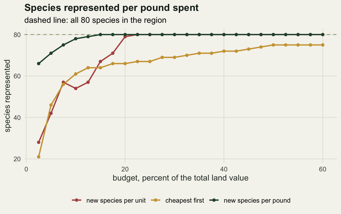
When does costing the land pay off?
The gain from dividing by price should depend on how price and biodiversity are arranged relative to each other. Varying the mixing weight moves the price surface from strongly negative to strongly positive correlation with richness while the species data, and the set of prices, stay exactly as they were.
The measure below is the gain: species under the benefit-cost rule divided by species under the cost-blind rule, at the same budget, so a value of 1.000 means accounting for price bought nothing. It is computed at two budgets, because the answer depends on that choice in a way worth seeing.
links <- c(-0.92, -0.5, 0, 0.5, 0.92)
sweep_df <- do.call(rbind, lapply(links, function(k) {
  rg <- make_region(price_link = k)
  tt <- sum(rg$price)
  blind_full <- greedy_plan(rg$pres, rg$price, Inf, "benefit")$spent / tt
  do.call(rbind, lapply(c(0.02, 0.15), function(f) {
    a <- greedy_plan(rg$pres, rg$price, f * tt, "benefit")$species
    b <- greedy_plan(rg$pres, rg$price, f * tt, "ratio")$species
    data.frame(correlation = round(cor(rg$price, rg$rich,
                                       method = "spearman"), 3),
               budget_percent = 100 * f, cost_blind = a, benefit_cost = b,
               gain = round(b / a, 3),
               blind_full_percent = round(100 * blind_full, 2))
  }))
}))
print(sweep_df, row.names = FALSE)
correlation budget_percent cost_blind benefit_cost gain blind_full_percent
-0.717 2 80 80 1.000 0.91
-0.717 15 80 80 1.000 0.91
-0.371 2 80 80 1.000 1.03
-0.371 15 80 80 1.000 1.03
-0.070 2 64 80 1.250 3.15
-0.070 15 80 80 1.000 3.15
0.279 2 49 75 1.531 13.13
0.279 15 80 80 1.000 13.13
0.687 2 19 63 3.316 22.81
0.687 15 67 80 1.194 22.81cat("total land value, identical at every mixing weight:",
round(sum(make_region(price_link = -0.92)$price)),
round(sum(make_region(price_link = 0.92)$price)), "\n")total land value, identical at every mixing weight: 12839 12839 The direction is the one the argument predicts, and the size depends on the budget. At the 2 per cent budget the gain climbs from 1.000 at a correlation of -0.717, through 1.250 at a correlation of -0.070, to 3.316 at a correlation of 0.687. The middle value is the interesting one: with price and richness essentially uncorrelated, dividing by price still buys more species than ignoring it, because the spread of prices alone creates cheap units worth taking first. Correlation raises the gain; variance alone is enough to produce one.
At the 15 per cent budget the gain is 1.000 everywhere except the last point, where it is 1.194. The reason sits in the last column, which is what full representation costs the cost-blind rule. When cheap land is the biodiverse land, that rule buys cheap land by accident and finishes for 0.91 per cent of the region’s value, so even a 2 per cent budget is slack and there is nothing left to gain. The share rises to 3.15 per cent at zero correlation and 22.81 per cent at the strongest positive correlation, and only in that last case does a 15 per cent budget bind.
So the honest form of the claim is conditional. Accounting for cost pays when the budget genuinely binds, and how binding a given budget is depends on the same correlation. A plan with money to spare gains nothing from cost efficiency, and few real plans are that comfortable.
sweep_df$panel <- factor(paste("budget", sweep_df$budget_percent,
                               "percent of land value"),
                         levels = c("budget 2 percent of land value",
                                    "budget 15 percent of land value"))
budget_cols <- c(te_pal$forest, te_pal$clay)
names(budget_cols) <- levels(sweep_df$panel)

ggplot(sweep_df, aes(correlation, gain, colour = panel)) +
  geom_hline(yintercept = 1, linetype = "dashed", colour = te_pal$sage) +
  geom_line(linewidth = 0.9) +
  geom_point(size = 2.4) +
  scale_colour_manual(values = budget_cols, name = NULL) +
  scale_x_continuous(expand = expansion(mult = 0.08)) +
  labs(title = "The gain depends on how price and richness line up",
       subtitle = "dashed line: dividing by price bought nothing",
       x = "Spearman correlation, unit price against species richness",
       y = "gain in species represented") +
  theme_te() +
  theme(legend.position = "bottom")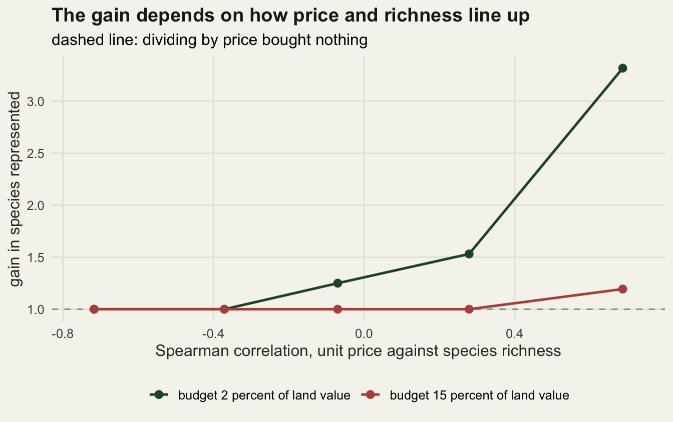
What the ratio rule cannot do
Two technical caveats first. Greedy selection on a ratio has no optimality guarantee, and an integer-programming formulation of the same budgeted problem will often find a cheaper set. Everything above measures one heuristic against two others, not the best achievable plan against them.
The second caveat is the data. No real analysis knows the price of a planning unit; it has a proxy, such as an asking price extrapolated from a few parcels, an opportunity cost derived from crop yields, or a management cost per hectare from an agency budget. Those proxies carry error, the error propagates straight into the ranking, and a ratio is more sensitive to error in its denominator than a sum is. The checking tutorial in this cluster puts numbers on that propagation.
Then the deeper problem, which the measurements above show rather than hide. Cheap land is usually cheap because nobody wants it, and land nobody wants is also land nobody is about to clear. The cost-only plan here bought units holding 0.87 species each; a cost-efficient plan drifts in that direction too, and a representation target cannot tell the difference between a species that is safe on cheap ground and a species that is one decision from losing its only site. Balmford and colleagues found the same bias in real reserve networks. Price, threat and biodiversity value are three separate axes, and this tutorial handles two.
Finally, the currency. Purchase price, forgone agricultural profit and annual management cost have different spatial patterns and produce different rankings. Choosing between them is a decision about what the plan is for, not a modelling step, and no analysis can make it for you.
Where to go next
Both plans in the first figure share a property this tutorial never measured: neither network is compact. The cost-blind selection is a scatter of near-isolated units, and the benefit-cost selection spreads 58 units across the region. Scattered reserves have more edge, cost more to manage per hectare, and support smaller local populations. The next tutorial adds a compactness penalty to the selection problem and measures what spatial coherence costs in species and in money.
References
Ando A, Camm J, Polasky S, Solow A 1998 Science 279(5359):2126-2128 (10.1126/science.279.5359.2126)
Balmford A, Gaston KJ, Blyth S, James A, Kapos V 2003 Proceedings of the National Academy of Sciences 100(3):1046-1050 (10.1073/pnas.0236945100)
Naidoo R et al 2006 Trends in Ecology and Evolution 21(12):681-687 (10.1016/j.tree.2006.10.003)
Murdoch W et al 2007 Biological Conservation 139(3-4):375-388 (10.1016/j.biocon.2007.07.011)