library(ggplot2)

te_pal <- list(forest = "#275139", green = "#2f8f63", sage = "#93a87f",
               clay = "#b5534e", gold = "#cda23f", line = "#dad9ca",
               ink = "#16241d", paper = "#f5f4ee")

theme_te <- function() {
  theme_minimal(base_size = 12) +
    theme(panel.grid.minor = element_blank(),
          panel.grid.major = element_line(colour = "#e7e6dc"),
          plot.background = element_rect(fill = "#f5f4ee", colour = NA),
          panel.background = element_rect(fill = "#f5f4ee", colour = NA),
          plot.title = element_text(face = "bold", colour = te_pal$ink),
          axis.title = element_text(colour = "#2c3a31"))
}Compactness in reserve design
R
conservation planning
optimisation
ecology tutorial
ggplot2
Add a boundary length penalty to a reserve selection problem in R, anneal it by hand, and measure what spatial cohesion really costs in conservation budget.
Greedy complementarity picks the planning unit that adds the most unrepresented species, and adding cost picks the unit that adds the most species per pound. Both produce the same awkward output: a scatter of single cells across the map. Nobody manages a reserve like that. Each cell carries its own access agreement, its own fence and its own patrol, and a one-cell reserve is entirely edge.
Marxan and the tools around it fix this by putting a spatial term in the objective and paying for it out of the same budget. The objective is the cost of the selected units, plus a boundary length modifier (BLM) times the boundary length of the selected set, plus a penalty for every species left below its target. This tutorial writes that objective out, minimises it with a hand-rolled annealer, and measures the exchange rate: how much conservation budget a unit of spatial cohesion actually costs.
Planning units, species and cost
A 20 by 20 grid of planning units, 60 species whose ranges are clustered blobs from smoothed random fields, and an acquisition cost surface that is also spatially structured and partly follows the same broad gradient the species do. That last detail matters: cheap land and species-rich land are not the same land, which is what makes the problem interesting.
Targets are proportional rather than token: each species needs at least 30 per cent of its occupied units inside the reserve. A one-unit or two-unit target makes the problem too easy to be worth a spatial term, because the whole solution is then a handful of cells and the cheapest arrangement of a handful of cells is already almost as compact as it can get.
smooth_field <- function(n, passes) {
  z <- matrix(runif(n * n), n, n)
  for (p in seq_len(passes)) {
    pad <- rbind(z[1, ], z, z[n, ])
    pad <- cbind(pad[, 1], pad, pad[, n])
    z <- (pad[1:n, 2:(n + 1)] + pad[3:(n + 2), 2:(n + 1)] +
            pad[2:(n + 1), 1:n] + pad[2:(n + 1), 3:(n + 2)] +
            4 * pad[2:(n + 1), 2:(n + 1)]) / 8
  }
  (z - min(z)) / (max(z) - min(z))
}

n_side <- 20L
n_unit <- n_side * n_side
n_spp <- 60L
penalty <- 1000

set.seed(5301)
gradient <- as.vector(smooth_field(n_side, 12))
rough <- as.vector(smooth_field(n_side, 6))
blend <- 0.5 * gradient + 0.5 * rough
unit_cost <- 1 + 19 * (blend - min(blend)) / diff(range(blend))

occ <- matrix(FALSE, n_unit, n_spp)
for (j in seq_len(n_spp)) {
  blob <- as.vector(smooth_field(n_side, 4)) * (1 + gradient)
  occ[, j] <- blob >= quantile(blob, 1 - runif(1, 0.05, 0.15))
}
richness <- rowSums(occ)
range_size <- colSums(occ)
target_share <- 0.3
target <- ceiling(target_share * range_size)

cat("planning units:", n_unit, " species:", n_spp, "\n")
planning units: 400 species: 60 cat("range size in units: min", min(range_size), " median",
median(range_size), " max", max(range_size), "\n")range size in units: min 22 median 39 max 60 cat("mean species per unit:", round(mean(richness), 2),
" units holding none of the 60:", sum(richness == 0), "\n")mean species per unit: 5.98 units holding none of the 60: 26 cat("acquisition cost per unit: min", round(min(unit_cost), 2),
" max", round(max(unit_cost), 2),
" whole region:", round(sum(unit_cost), 1), "\n")acquisition cost per unit: min 1 max 20 whole region: 4293.1 cat("penalty per species left below target:", penalty,
" most expensive unit on the map:", round(max(unit_cost), 2), "\n")penalty per species left below target: 1000 most expensive unit on the map: 20 cat("correlation between cost and species richness:",
round(cor(unit_cost, richness), 4), "\n")correlation between cost and species richness: 0.6323 cat("target share of each range:", 100 * target_share,
"percent\n")target share of each range: 30 percentcat("target occurrences per species: min", min(target), " median",
median(target), " max", max(target), " summed:", sum(target), "\n")target occurrences per species: min 7 median 12 max 18 summed: 745 Ranges run from 22 to 60 units with a median of 39, so a unit holds 5.98 species on average and only 26 of the 400 hold none of them. The targets add up to 745 occurrences that have to be found somewhere. Cost and richness correlate at 0.6323, which is the usual conservation problem in miniature: the land worth protecting is the land somebody else wants.
The objective, written out
Three terms, all in the same currency.
The cost term is the sum of unit_cost over the selected units. The representation term is the penalty times the number of species below target, with the penalty set to 1000, far above the cost of the few units that would fix any single shortfall, so a solution that drops a species is never competitive.
The boundary term needs a convention, and the convention changes the numbers, so it should be stated rather than assumed. Here every planning unit has four edges of length one, and an edge counts towards the boundary if the unit across it is not selected. Units on the margin of the grid are treated as bordering unselected land, so their outer edges count too. In code that is a phantom extra unit beyond the 400, permanently unselected. A single unit alone therefore scores 4, two units side by side score 6, and a solid 6 by 6 block scores 24, its perimeter.
outside <- n_unit + 1L
nb_up <- integer(n_unit)
nb_down <- integer(n_unit)
nb_left <- integer(n_unit)
nb_right <- integer(n_unit)
for (u in seq_len(n_unit)) {
  y <- ((u - 1L) %% n_side) + 1L
  x <- ((u - 1L) %/% n_side) + 1L
  nb_up[u] <- if (y > 1L) u - 1L else outside
  nb_down[u] <- if (y < n_side) u + 1L else outside
  nb_left[u] <- if (x > 1L) u - n_side else outside
  nb_right[u] <- if (x < n_side) u + n_side else outside
}
spp_at <- lapply(seq_len(n_unit), function(u) which(occ[u, ]))

boundary_length <- function(sel) {
  pad <- c(sel, FALSE)
  kept <- pad[nb_up] + pad[nb_down] + pad[nb_left] + pad[nb_right]
  sum((4L - kept)[sel])
}

shortfall <- function(sel) sum(colSums(occ[sel, , drop = FALSE]) < target)

objective <- function(sel, blm) {
  sum(unit_cost[sel]) + blm * boundary_length(sel) + penalty * shortfall(sel)
}

count_clusters <- function(sel) {
  pad <- c(sel, FALSE)
  label <- integer(n_unit + 1L)
  found <- 0L
  for (u in which(sel)) {
    if (label[u] > 0L) next
    found <- found + 1L
    queue <- u
    while (length(queue) > 0L) {
      v <- queue[length(queue)]
      queue <- queue[-length(queue)]
      if (label[v] > 0L) next
      label[v] <- found
      side <- c(nb_up[v], nb_down[v], nb_left[v], nb_right[v])
      queue <- c(queue, side[pad[side] & label[side] == 0L])
    }
  }
  found
}

block <- matrix(FALSE, n_side, n_side)
block[6:11, 6:11] <- TRUE
lone <- rep(FALSE, n_unit)
lone[45] <- TRUE
pair <- lone
pair[46] <- TRUE
apart <- lone
apart[200] <- TRUE
cat("boundary length of one unit:", boundary_length(lone),
    " of two adjacent units:", boundary_length(pair),
    " of a solid 6 by 6 block:", boundary_length(as.vector(block)), "\n")
boundary length of one unit: 4 of two adjacent units: 6 of a solid 6 by 6 block: 24 cat("clusters in that block:", count_clusters(as.vector(block)),
" in two cells far apart:", count_clusters(apart), "\n")clusters in that block: 1 in two cells far apart: 2 count_clusters is a flood fill on the rook neighbourhood, and it is the diagnostic the boundary term is really aiming at: how many separate pieces the reserve has.
The flip that makes it affordable
Simulated annealing proposes a change, accepts it if the objective falls, and accepts it with probability exp(-delta / temperature) if it rises, with the temperature cooling geometrically so that the search starts as a random walk and ends as hill descent. The proposal here is the simplest one: pick a planning unit at random and flip its status.
The only reason a run of a quarter of a million flips is affordable in R is that the change in the objective can be worked out from the flipped unit alone.
Cost changes by plus or minus that unit’s own cost. Boundary length changes by a term that only involves the unit’s four neighbours: if k of them are selected, turning the unit on adds its own 4 - k exposed edges and removes the k edges its selected neighbours were exposing towards it, for a net change of 4 - 2k, and turning it off changes the sign. Representation changes only for the species present in that unit: switching on can only rescue a species whose count sits exactly one below its target, and switching off can only break a species sitting exactly on it.
n_iter <- 250000L

anneal <- function(blm, start, iters, t_hot, t_cold, thin = 250L) {
  pad <- c(start, FALSE)
  cnt <- colSums(occ[start, , drop = FALSE])
  money <- sum(unit_cost[start])
  edges <- boundary_length(start)
  short <- sum(cnt < target)
  obj <- money + blm * edges + penalty * short
  picks <- sample.int(n_unit, iters, replace = TRUE)
  gate <- t_hot * (t_cold / t_hot)^(seq_len(iters) / iters) *
    (-log(runif(iters)))
  obj_trace <- numeric(iters %/% thin)
  for (it in seq_len(iters)) {
    u <- picks[it]
    flip <- if (pad[u]) -1L else 1L
    kept <- pad[nb_up[u]] + pad[nb_down[u]] + pad[nb_left[u]] + pad[nb_right[u]]
    d_edges <- flip * (4L - 2L * kept)
    here <- spp_at[[u]]
    d_short <- 0L
    if (length(here) > 0L) {
      d_short <- if (flip > 0L) -sum(cnt[here] == target[here] - 1L) else
        sum(cnt[here] == target[here])
    }
    delta <- flip * unit_cost[u] + blm * d_edges + penalty * d_short
    if (delta < gate[it]) {
      pad[u] <- !pad[u]
      if (length(here) > 0L) cnt[here] <- cnt[here] + flip
      money <- money + flip * unit_cost[u]
      edges <- edges + d_edges
      short <- short + d_short
      obj <- obj + delta
    }
    if (it %% thin == 0L) obj_trace[it %/% thin] <- obj
  }
  list(sel = pad[seq_len(n_unit)], obj = obj, cost = money, boundary = edges,
       shortfall = short, obj_trace = obj_trace)
}

cat("iterations per run:", n_iter, "\n")
iterations per run: 250000 cat("occurrence entries a full evaluation reads:", n_unit * n_spp,
" an incremental flip reads on average:", round(mean(richness), 2), "\n")occurrence entries a full evaluation reads: 24000 an incremental flip reads on average: 5.98 The acceptance test is folded into one comparison. Instead of drawing a uniform and comparing it with exp(-delta / temperature), the whole schedule is precomputed as temperature times -log(uniform), and a move is accepted when delta falls below that gate. Downhill moves pass automatically because the gate is always positive.
A full evaluation of the objective reads all 24000 entries of the occurrence matrix; an incremental flip reads the 5.98 species in one unit, on average, plus four neighbours. Multiply that by the 250000 iterations in every run, and by the runs the sweep below needs, and the difference is the difference between a page that knits and one that does not.
One run, and a check on the arithmetic
Tracking an objective incrementally invites drift, so the first thing to do with a run is score its answer from scratch and compare.
set.seed(5302)
solo <- anneal(4, runif(n_unit) < 0.4, n_iter, 72, 0.05)
cat("objective carried incrementally:", round(solo$obj, 3), "\n")
objective carried incrementally: 1673.431 cat("the same solution scored from scratch:",
round(objective(solo$sel, 4), 3),
" difference:", round(solo$obj - objective(solo$sel, 4), 10), "\n")the same solution scored from scratch: 1673.431 difference: 0 cat("units selected:", sum(solo$sel), " cost", round(solo$cost, 1),
" boundary", solo$boundary, " species below target:", solo$shortfall,
" clusters:", count_clusters(solo$sel), "\n")units selected: 82 cost 937.4 boundary 184 species below target: 0 clusters: 20 The two agree to the last digit, difference 0, which is the check worth writing into any annealer: if the incremental bookkeeping is wrong, the search optimises something other than the objective and the output still looks plausible. This run, at BLM 4, buys 82 units for a cost of 937.4 with a boundary of 184, and meets all 60 targets.
What compactness costs
Now sweep the BLM from zero upwards. Each point is the best of three annealing runs from independent random starts, which is standard practice and, as the comparison just below shows, necessary.
blm_grid <- c(0, 1, 2, 4, 8, 16, 32)
set.seed(5303)
runs <- lapply(blm_grid, function(b) {
  best <- NULL
  for (attempt in 1:3) {
    r <- anneal(b, runif(n_unit) < 0.4, n_iter, 40 + 8 * b, 0.05)
    if (is.null(best) || r$obj < best$obj) best <- r
  }
  best
})

blm_tab <- data.frame(
  blm = blm_grid,
  objective = round(sapply(runs, function(r) r$obj), 1),
  cost = round(sapply(runs, function(r) r$cost), 1),
  boundary = sapply(runs, function(r) r$boundary),
  units = sapply(runs, function(r) sum(r$sel)),
  clusters = sapply(runs, function(r) count_clusters(r$sel)),
  unmet = sapply(runs, function(r) r$shortfall))
print(blm_tab, row.names = FALSE)
blm objective cost boundary units clusters unmet
0 932.9 932.9 248 86 41 0
1 1170.1 954.1 216 88 27 0
2 1317.5 937.5 190 82 18 0
4 1603.8 971.8 158 86 14 0
8 2110.7 1070.7 130 95 10 0
16 2806.4 1270.4 96 104 4 0
32 3900.1 1596.1 72 121 2 0Three starts already earn their keep. At BLM 4 the best of the three reaches an objective of 1603.8, against 1673.431 for the single run above.
value <- data.frame(
  blm = blm_grid,
  cost_rise_pc = round(100 * (blm_tab$cost / blm_tab$cost[1] - 1), 1),
  boundary_drop_pc = round(100 * (1 - blm_tab$boundary / blm_tab$boundary[1]), 1),
  edges_per_extra_cost = round((blm_tab$boundary[1] - blm_tab$boundary) /
                                 (blm_tab$cost - blm_tab$cost[1]), 2))
print(value[-1, ], row.names = FALSE)
blm cost_rise_pc boundary_drop_pc edges_per_extra_cost
1 2.3 12.9 1.51
2 0.5 23.4 12.61
4 4.2 36.3 2.31
8 14.8 47.6 0.86
16 36.2 61.3 0.45
32 71.1 71.0 0.27cx <- (blm_tab$cost - min(blm_tab$cost)) / diff(range(blm_tab$cost))
cy <- (blm_tab$boundary - min(blm_tab$boundary)) / diff(range(blm_tab$boundary))
knee <- which.max(abs(cx + cy - 1) / sqrt(2))
cat("knee of the curve at BLM", blm_tab$blm[knee], ": boundary down",
value$boundary_drop_pc[knee], "percent for",
value$cost_rise_pc[knee], "percent more money\n")knee of the curve at BLM 8 : boundary down 47.6 percent for 14.8 percent more moneycat("last step, BLM 16 to 32: boundary down",
round(100 * (1 - blm_tab$boundary[7] / blm_tab$boundary[6]), 1),
"percent for", round(100 * (blm_tab$cost[7] / blm_tab$cost[6] - 1), 1),
"percent more money\n")last step, BLM 16 to 32: boundary down 25 percent for 25.6 percent more moneycat("percent of the region selected at BLM 0, 8 and 32:",
round(100 * blm_tab$units[c(1, 5, 7)] / n_unit, 2), "\n")percent of the region selected at BLM 0, 8 and 32: 21.5 23.75 30.25 The first slice of compactness is nearly free. Going from BLM 0 to BLM 2 removes 23.4 per cent of the boundary for 0.5 per cent more money, and it cuts the reserve from 41 separate clusters to 18. At BLM 4 the boundary is down 36.3 per cent for 4.2 per cent more money. Those two rows are the reason a spatial term belongs in the objective at all: the cost-only solution was paying nothing for its scatter, and a small weight rearranges the same money into something a manager can walk around.
Then the price appears. The edges_per_extra_cost column is the exchange rate, edges removed per unit of extra acquisition cost, and it falls from 12.61 at BLM 2 to 0.86 at BLM 8 and 0.27 at BLM 32. The knee of the curve, the point furthest from the chord joining its ends, sits at BLM 8: boundary down 47.6 per cent for 14.8 per cent more money. After that each further improvement is bought at close to full price. The last step, BLM 16 to BLM 32, removes 25 per cent more boundary for 25.6 per cent more money, and it does that by buying 121 units instead of 104, so the reserve grows from 21.5 per cent of the region at BLM 0 to 30.25 per cent at BLM 32.
panels <- c(1, knee, length(blm_grid))
map_df <- do.call(rbind, lapply(panels, function(i) {
  data.frame(x = rep(seq_len(n_side), each = n_side),
             y = rep(seq_len(n_side), times = n_side),
             species = richness,
             chosen = runs[[i]]$sel,
             panel = sprintf("BLM %g: %d edges, %d clusters",
                             blm_tab$blm[i], blm_tab$boundary[i],
                             blm_tab$clusters[i]))
}))
map_df$panel <- factor(map_df$panel, levels = unique(map_df$panel))

ggplot(map_df, aes(x, y)) +
  geom_raster(aes(fill = species)) +
  geom_raster(data = subset(map_df, chosen), fill = te_pal$clay, alpha = 0.85) +
  facet_wrap(~panel, nrow = 1) +
  coord_equal() +
  scale_fill_gradient(low = te_pal$paper, high = te_pal$forest,
                      name = "species") +
  labs(title = "Confetti, blocks, blob",
       subtitle = "red: selected units, green: species richness of the region",
       x = NULL, y = NULL) +
  theme_te() +
  theme(axis.text = element_blank(), panel.grid = element_blank())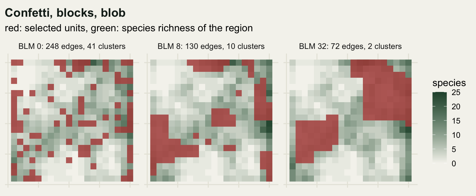
The third panel is where the argument turns around. That reserve is cohesive and it meets every target, but it holds 30.25 per cent of the region and pays 71.1 per cent more than the scattered solution for the same species list. Cohesion has stopped being a design improvement and become the design.
ggplot(blm_tab, aes(cost, boundary)) +
  geom_path(colour = te_pal$sage, linewidth = 0.9) +
  geom_point(colour = te_pal$forest, size = 2.8) +
  geom_text(aes(label = paste("BLM", blm)), hjust = -0.16, vjust = -0.5,
            colour = te_pal$ink, size = 3.3) +
  expand_limits(x = max(blm_tab$cost) * 1.1, y = max(blm_tab$boundary) + 12) +
  labs(title = "Compactness is cheap, then it is not",
       subtitle = "each point is the best of three annealing runs at one BLM",
       x = "total acquisition cost of the selected units",
       y = "boundary length (edges)") +
  theme_te()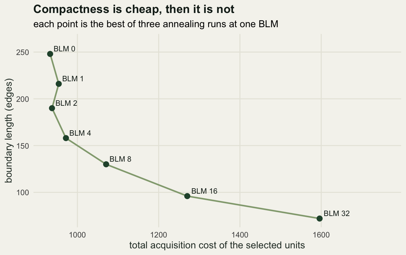
Eight starts, eight reserves
One curve from one optimiser is not a result yet. Run the knee BLM again from eight independent random starts and look at what comes back.
knee_blm <- blm_tab$blm[knee]
set.seed(5304)
reps <- lapply(seq_len(8), function(i)
  anneal(knee_blm, runif(n_unit) < 0.4, n_iter, 40 + 8 * knee_blm, 0.05))
rep_obj <- sapply(reps, function(r) r$obj)
cat("eight starts at BLM", knee_blm, ": best objective", round(min(rep_obj), 1),
    " worst", round(max(rep_obj), 1),
    " worst over best:", round(max(rep_obj) / min(rep_obj), 4), "\n")
eight starts at BLM 8 : best objective 2079.8 worst 2252.2 worst over best: 1.0829 cat("units selected in each run:", sapply(reps, function(r) sum(r$sel)), "\n")units selected in each run: 85 92 91 86 93 83 86 92 cat("runs that missed a target:",
sum(sapply(reps, function(r) r$shortfall) > 0), "\n")runs that missed a target: 0 overlap <- function(a, b) sum(a & b) / sum(a | b)
pair_ov <- numeric(0)
for (i in 1:7) {
for (j in (i + 1):8) {
pair_ov <- c(pair_ov, overlap(reps[[i]]$sel, reps[[j]]$sel))
}
}
cat("mean pairwise overlap:", round(mean(pair_ov), 4),
" lowest", round(min(pair_ov), 4), " highest", round(max(pair_ov), 4), "\n")mean pairwise overlap: 0.3631 lowest 0.2158 highest 0.5164 picked <- rowSums(sapply(reps, function(r) r$sel))
cat("units chosen by all eight runs:", sum(picked == 8L),
" by at least one:", sum(picked > 0L),
" by exactly one:", sum(picked == 1L), "\n")units chosen by all eight runs: 10 by at least one: 209 by exactly one: 52 Every run meets every target and the objectives are close, the worst only 1.0829 times the best. The best of the eight, 2079.8, is itself better than the 2110.7 the sweep recorded at this BLM, so even the curve is drawn from good solutions rather than optimal ones. The maps are not close at all. Mean pairwise overlap, measured as shared units over units in either solution, is 0.3631, with the most similar pair at 0.5164 and the least similar at 0.2158. Across the eight runs 209 different units get selected at least once, 52 of them by exactly one run, and only 10 are chosen by all eight.
trace_df <- do.call(rbind, lapply(seq_along(reps), function(i) {
  tr <- reps[[i]]$obj_trace
  data.frame(iteration = seq_along(tr) * 250,
             objective = tr, run = paste("start", i))
}))

ggplot(trace_df, aes(iteration, objective, group = run)) +
  geom_line(colour = te_pal$forest, alpha = 0.65, linewidth = 0.5) +
  scale_y_log10() +
  scale_x_continuous(labels = function(v) format(v, big.mark = " ")) +
  labs(title = "Eight starts, eight different reserves",
       subtitle = sprintf("BLM %g, mean pairwise overlap %.2f",
                          knee_blm, mean(pair_ov)),
       x = "iteration", y = "objective (log scale)") +
  theme_te()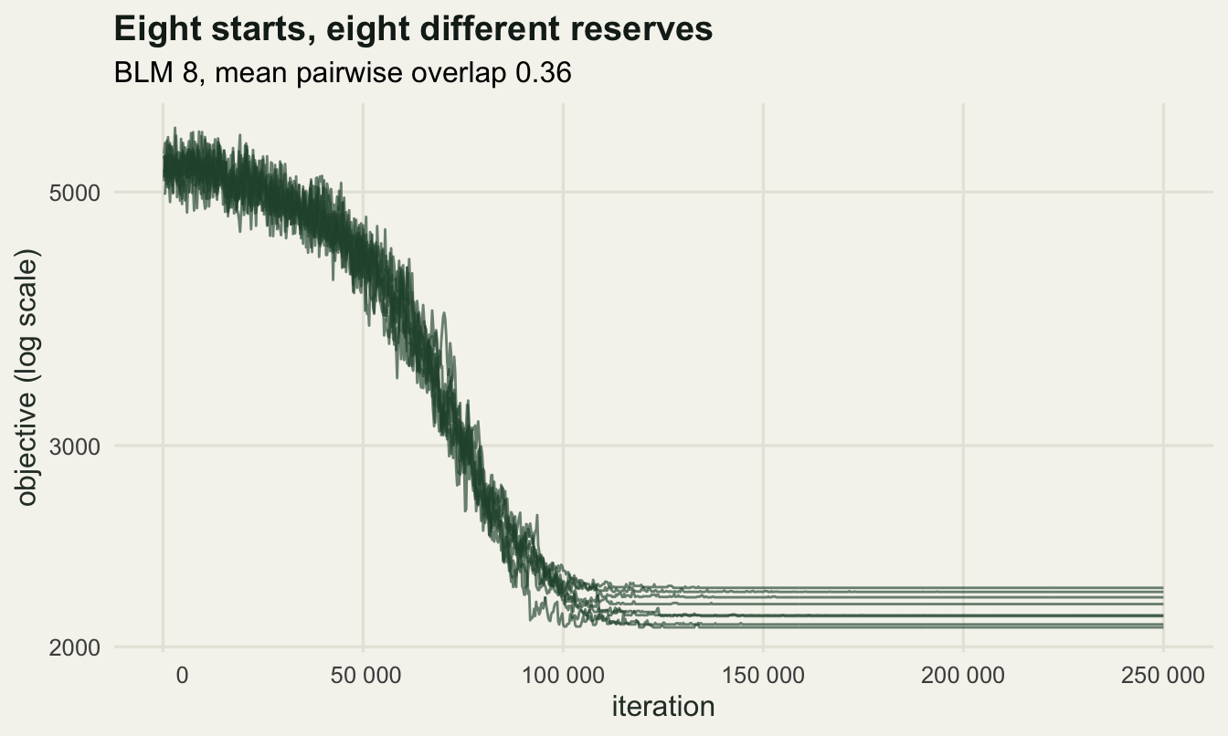
That is the case against handing anyone a single map. Eight equally good answers to the same question disagree about two thirds of their content, and nothing in the objective distinguishes them. The 10 units every run selected are a different kind of finding from the 52 that one run selected once; a single solution map hides the difference, and the next tutorial turns it into selection frequency.
What the boundary term does not model
Boundary length is a proxy for spatial cohesion and nothing more. It has no notion of what crosses the edge, so it cannot distinguish a boundary against arable land from a boundary against continuous forest, and the usual fix, weighting each edge by what lies across it, is a data problem rather than a modelling one. It is not a connectivity model either: two blocks joined by a narrow corridor score worse than a single blob of the same area, because the corridor adds edges, even when the corridor is the thing the species needs. If connectivity is the actual objective, it has to be measured as connectivity, with the metrics in the least-cost path and circuit theory tutorials, and the fragmentation tutorial covers what patch shape does to edge exposure.
The BLM itself has no correct value. It is an exchange rate between money and cohesion, chosen by the analyst, and the sweep above shows that the choice moves the answer from 41 clusters to 2 and the budget by 71.1 per cent. So the BLM belongs in the sensitivity analysis, reported as a curve, not buried in a defaults file with the number 1 next to it.
Annealing gives a good solution, not the optimum. The evidence is in the sweep table itself: cost at BLM 1 came out at 954.1, higher than the 937.5 at BLM 2, and an exact optimiser cannot do that, because a larger weight on boundary length can never lower the cost of the optimal solution. That wobble is the optimiser’s error bar showing through, the same thing the 1.0829 spread between the eight restarts measures directly.
Where to go next
The next tutorial in this cluster takes the eight disagreeing maps seriously and builds the checks a prioritisation needs before it leaves the laptop: selection frequency across many runs instead of one solution, sensitivity of the answer to the targets, sensitivity to the cost layer, and what happens to all of it when a few units are locked in or locked out by decisions that were made before the analysis started.
References
Possingham HP, Ball IR, Andelman S 2000 in Ferson S, Burgman MA (eds) Quantitative Methods for Conservation Biology, Springer, ISBN 978-0387943220
McDonnell MD, Possingham HP, Ball IR, Cousins EA 2002 Environmental Modeling and Assessment 7(2):107-114 (10.1023/A:1015649716111)
Fischer DT, Church RL 2003 Forest Science 49(4):555-565 (10.1093/forestscience/49.4.555)
Watts ME et al 2009 Environmental Modelling and Software 24(12):1513-1521 (10.1016/j.envsoft.2009.06.005)
Moilanen A, Wilson KA, Possingham HP (eds) 2009 Spatial Conservation Prioritization, Oxford University Press, ISBN 978-0199547760