library(ggplot2)

te_pal <- list(forest = "#275139", green = "#2f8f63", sage = "#93a87f",
               clay = "#b5534e", gold = "#cda23f", line = "#dad9ca",
               ink = "#16241d", paper = "#f5f4ee")

theme_te <- function() {
  theme_minimal(base_size = 12) +
    theme(panel.grid.minor = element_blank(),
          panel.grid.major = element_line(colour = "#e7e6dc"),
          plot.background = element_rect(fill = "#f5f4ee", colour = NA),
          panel.background = element_rect(fill = "#f5f4ee", colour = NA),
          plot.title = element_text(face = "bold", colour = te_pal$ink),
          axis.title = element_text(colour = "#2c3a31"))
}
The expected value of information
R
conservation
decision analysis
ecology tutorial
ggplot2
Compute the expected value of perfect, partial and sample information by hand in R for a conservation decision, and measure when uncertainty is worth nothing.
Every conservation programme has a queue of things it does not know. A reserve manager watching breeding waders decline can tell you within a minute which unknowns keep them awake: whether the losses are predation or habitat, whether restoration will deliver inside the funding window, whether the count is even right. The natural next move is to rank those unknowns by how uncertain they are and send the survey budget after the biggest one.
That ranking is wrong, and it is wrong in a way that has a clean proof. Information has value only through the decision it changes. An unknown that leaves the best action the same, whatever its value turns out to be, is worth exactly nothing to resolve, no matter how uncertain it is. An unknown you are nearly sure about can be worth a great deal, if the small residual doubt sits across the line where one action overtakes another. The arithmetic that makes this precise is the expected value of information, and it is small enough to write from scratch.
This post codes it by hand on one decision: a wet grassland reserve losing breeding lapwing, three management alternatives, and four uncertain quantities with stated priors. We compute the expected value of perfect information, then the partial value of resolving each unknown alone, then the value of a real survey with imperfect sensitivity and specificity, and finally what happens to the total when a new alternative joins the set. If the framing of alternatives, states and consequences is unfamiliar, structured decision making in R builds the table this post prices.
Nothing here is quoted. Every value is computed in the code on this page, and where the answer contradicts the intuition, the answer stays.
The decision
A lowland wet grassland reserve holds breeding lapwing. Counts have fallen at roughly five per cent a year and the reserve has one management budget to spend for the next planning cycle. The consequence we score is the number of breeding pairs projected at the end of that cycle. Three alternatives are on the table at the start: carry on monitoring and change nothing, run predator control over the whole reserve, or restore the sward and the surface water regime.
Four things are uncertain, and each has a prior the reserve staff would recognise as their own.
The driver of the decline is either nest predation or habitat condition. That is not a binary in nature, so it is coded as which of the two carries the larger share of the annual deficit in growth rate. The lag on restoration says whether a restored sward delivers inside the planning horizon or arrives late, because water level control takes several seasons to bed in. The rebound of predators says whether controlled foxes and corvids are replaced quickly from the surrounding farmland or slowly. The census is the current number of pairs, which nobody knows to better than a wide bracket, because lapwing are counted by territory mapping on a site with poor sightlines.
The outcome model is a single exponential trend. The population declines at a fixed rate, each alternative removes some part of the deficit that its target driver contributes, and the projected count at the horizon is the current count multiplied by the compounded trend. The two efficiency parameters convert an alternative into a recovered fraction of its own deficit share.
horizon <- 15
r_decline <- -0.048

cause_lv <- c("predation", "habitat");   cause_pr <- c(0.55, 0.45)
lag_lv   <- c("on time", "delayed");     lag_pr   <- c(0.88, 0.12)
reb_lv   <- c("slow", "fast");           reb_pr   <- c(0.60, 0.40)
cen_lv   <- c(110, 145, 185);            cen_pr   <- c(0.30, 0.45, 0.25)

pred_share <- c(predation = 0.035, habitat = 0.010)
hab_share  <- c(predation = 0.013, habitat = 0.038)
eff_pred   <- c(slow = 0.90, fast = 0.30)
eff_hab    <- c("on time" = 0.90, delayed = 0.20)

states <- expand.grid(cause = cause_lv, lag = lag_lv, rebound = reb_lv,
                      census = cen_lv, stringsAsFactors = FALSE)
states$prob <- cause_pr[match(states$cause, cause_lv)] *
  lag_pr[match(states$lag, lag_lv)] *
  reb_pr[match(states$rebound, reb_lv)] *
  cen_pr[match(states$census, cen_lv)]

entropy <- function(p) -sum(p * log(p))
ent_prior <- c(cause = entropy(cause_pr), lag = entropy(lag_pr),
               rebound = entropy(reb_pr), census = entropy(cen_pr))

print(c(states = nrow(states), total_probability = sum(states$prob),
        horizon_years = horizon, annual_decline = -r_decline,
        mean_census = sum(cen_pr * cen_lv)))
states total_probability horizon_years annual_decline
24.000 1.000 15.000 0.048
mean_census
144.500 print(c(census_levels = cen_lv, census_prior = cen_pr))census_levels1 census_levels2 census_levels3 census_prior1 census_prior2
110.00 145.00 185.00 0.30 0.45
census_prior3
0.25 print(c(cause_prior = cause_pr, lag_prior = lag_pr, rebound_prior = reb_pr)) cause_prior1 cause_prior2 lag_prior1 lag_prior2 rebound_prior1
0.55 0.45 0.88 0.12 0.60
rebound_prior2
0.40 print(round(ent_prior, 4)) cause lag rebound census
0.6881 0.3669 0.6730 1.0671 Twenty four states, because the four quantities are taken as independent and multiply out to 2 times 2 times 2 times 3. The horizon is 15 years and the untreated decline is 0.048 a year. The census prior puts 0.3 on 110 pairs, 0.45 on 145 and 0.25 on 185, for a prior mean of 144.5.
The entropies of the four priors are printed in nats and they set up the whole post. The census is by far the most uncertain quantity at 1.0671, because it has three levels and none of them is favoured much. The driver follows at 0.6881 and the predator rebound at 0.673. The restoration lag is the quantity the reserve is most confident about, at 0.3669: they are 88 per cent sure the restoration lands on time. Remember that ordering. It is the ordering a workshop would use to allocate a monitoring budget.
gain_pred <- as.numeric(eff_pred[states$rebound] * pred_share[states$cause])
gain_hab  <- as.numeric(eff_hab[states$lag] * hab_share[states$cause])
gains <- cbind(monitor = 0 * gain_pred, predator = gain_pred, habitat = gain_hab)
payoff <- states$census * exp(horizon * (r_decline + gains))
colnames(payoff) <- colnames(gains)

core <- interaction(states$cause, states$lag, states$rebound, drop = TRUE)
state_table <- do.call(rbind, lapply(split(seq_len(nrow(states)), core), function(i)
  colSums(states$prob[i] * payoff[i, , drop = FALSE]) / sum(states$prob[i])))
print(round(state_table, 2))
monitor predator habitat
habitat.delayed.fast 70.34 73.57 78.83
predation.delayed.fast 70.34 82.33 73.13
habitat.on time.fast 70.34 73.57 117.48
predation.on time.fast 70.34 82.33 83.83
habitat.delayed.slow 70.34 80.50 78.83
predation.delayed.slow 70.34 112.82 73.13
habitat.on time.slow 70.34 80.50 117.48
predation.on time.slow 70.34 112.82 83.83The table above averages over the census, which is why it has eight rows rather than 24. Read one row: when predation drives the decline, restoration is delayed and predators rebound slowly, predator control projects 112.82 pairs against 73.13 for restoration and 70.34 for doing nothing. Move to the row where habitat drives the decline and restoration lands on time, and the ranking inverts: 117.48 pairs for restoration against 80.5 for predator control. Doing nothing returns 70.34 in every row, because the census cancels out of the comparison and no management means no recovered deficit.
sp <- do.call(rbind, strsplit(rownames(state_table), ".", fixed = TRUE))
combo_lv <- c("slow, on time", "slow, delayed", "fast, on time", "fast, delayed")
plot_pay <- data.frame(
  cause = ifelse(sp[, 1] == "predation", "Driver: predation", "Driver: habitat"),
  combo = factor(paste(sp[, 3], sp[, 2], sep = ", "), levels = combo_lv),
  monitor = state_table[, "monitor"], predator = state_table[, "predator"],
  habitat = state_table[, "habitat"])
alt_lab <- c(monitor = "Monitor only", predator = "Predator control",
             habitat = "Habitat restoration")
long_pay <- do.call(rbind, lapply(names(alt_lab), function(a)
  data.frame(cause = plot_pay$cause, combo = plot_pay$combo,
             value = as.numeric(plot_pay[[a]]),
             alternative = unname(alt_lab[a]), row.names = NULL)))
long_pay$alternative <- factor(long_pay$alternative, levels = alt_lab)
long_pay$cause <- factor(long_pay$cause,
                         levels = c("Driver: predation", "Driver: habitat"))
env <- do.call(rbind, lapply(split(long_pay, list(long_pay$cause, long_pay$combo)),
                             function(z) z[which.max(z$value), ]))

ggplot(long_pay, aes(combo, value, colour = alternative, group = alternative)) +
  geom_line(linewidth = 0.8) +
  geom_point(size = 2.2) +
  geom_point(data = env, shape = 1, size = 5, stroke = 1.1, colour = te_pal$ink) +
  facet_wrap(~cause) +
  scale_colour_manual(values = c(te_pal$sage, te_pal$forest, te_pal$clay), name = NULL) +
  labs(x = "Predator rebound, restoration timing",
       y = "Projected pairs at year 15",
       title = "The best action changes with the state") +
  theme_te() +
  theme(legend.position = "top",
        strip.text = element_text(colour = te_pal$ink, face = "bold"))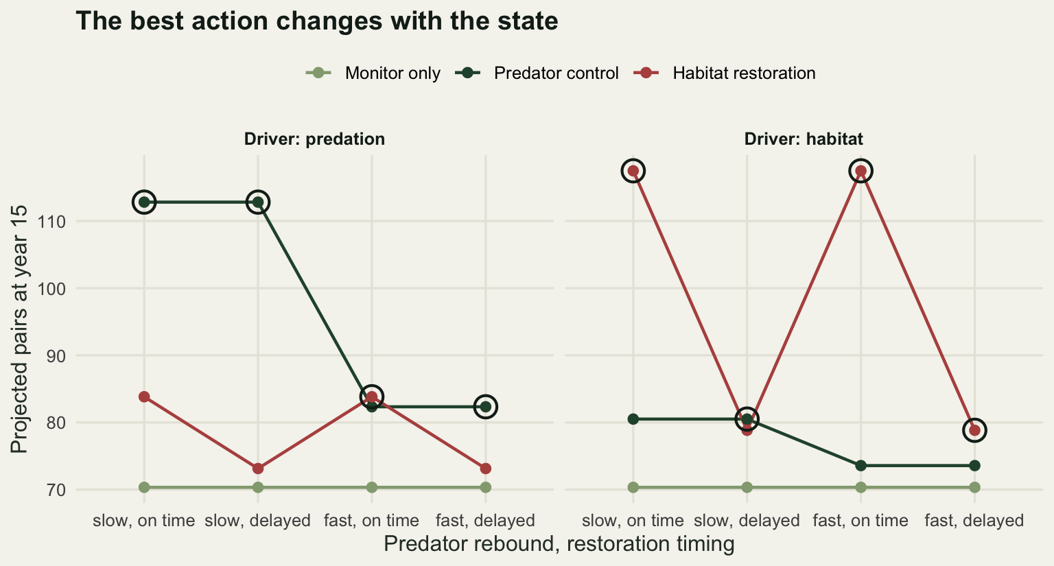
The baseline and the expected value of perfect information
Two numbers define everything that follows. The first is what the decision is worth now: take the prior weighted mean payoff of each alternative, and keep the largest. The second is what the decision would be worth to an analyst who was told the true state before choosing: take the best payoff within each state, then average those over the prior. The difference is the expected value of perfect information.
The order of the maximum and the average is the whole idea. The baseline is a maximum of averages. The informed value is an average of maxima. A maximum of averages can never beat an average of maxima, so the difference is never negative, and it is zero exactly when the same alternative wins the inner maximum every time.
evpi <- function(P, p) sum(p * apply(P, 1, max)) - max(colSums(p * P))

ev_prior <- colSums(states$prob * payoff)
ev_perfect <- sum(states$prob * apply(payoff, 1, max))
evpi_base <- evpi(payoff, states$prob)

print(round(ev_prior, 3))
monitor predator habitat
70.336 90.322 96.179 cat("best action under the prior:", names(ev_prior)[which.max(ev_prior)], "\n")best action under the prior: habitat print(round(c(best_expected_value = max(ev_prior),
value_under_perfect_information = ev_perfect,
evpi_pairs = evpi_base,
evpi_percent_of_baseline = 100 * evpi_base / max(ev_prior)), 3)) best_expected_value value_under_perfect_information
96.179 106.467
evpi_pairs evpi_percent_of_baseline
10.287 10.696 Under the prior, doing nothing projects 70.336 pairs, predator control 90.322 and restoration 96.179. Restoration is the best action and the reserve should take it today. An analyst who knew the state before choosing would average 106.467 pairs. The expected value of perfect information is therefore 10.287 pairs, which is 10.696 per cent of what the decision is already worth.
That is the number to negotiate over. It is a hard ceiling on any study, survey, pilot or expert elicitation aimed at this decision: not the ceiling on a well designed one, the ceiling on all of them, including a hypothetical study that returns the truth free of error and free of delay. If someone proposes research whose cost exceeds 10.287 pairs of projected population, the proposal is refuted before the methods section.
Uncertainty that is worth nothing
The headline claim of this post is that the size of an uncertainty tells you almost nothing about its value. The cleanest way to show it is to build two small decisions by hand, one with maximal uncertainty and no value, one with minimal uncertainty and real value.
The first has four states, each with probability one quarter, which is the highest entropy a four state prior can have. The payoffs across states range from 33 to 178 pairs, so the states matter enormously to the outcome. But one alternative is best in every state.
The second has two states with probabilities 0.97 and 0.03, which is a prior close to certainty. The two alternatives are nearly tied under it.
dom_pay <- cbind(monitor = c(40, 95, 62, 150),
                 predator = c(58, 121, 80, 178),
                 habitat = c(33, 88, 55, 141))
dom_pr <- rep(0.25, 4)

tie_pay <- cbind(monitor = c(100, 60), predator = c(99, 100))
tie_pr <- c(0.97, 0.03)

evpi_dom <- evpi(dom_pay, dom_pr)
evpi_tie <- evpi(tie_pay, tie_pr)

print(cbind(probability = dom_pr, dom_pay))
probability monitor predator habitat
[1,] 0.25 40 58 33
[2,] 0.25 95 121 88
[3,] 0.25 62 80 55
[4,] 0.25 150 178 141print(cbind(probability = tie_pr, tie_pay)) probability monitor predator
[1,] 0.97 100 99
[2,] 0.03 60 100print(round(colSums(dom_pr * dom_pay), 3)) monitor predator habitat
86.75 109.25 79.25 print(round(colSums(tie_pr * tie_pay), 3)) monitor predator
98.80 99.03 print(round(c(dominant_case_entropy = entropy(dom_pr), dominant_case_evpi = evpi_dom,
near_tie_entropy = entropy(tie_pr), near_tie_evpi = evpi_tie,
entropy_ratio = entropy(dom_pr) / entropy(tie_pr)), 4))dominant_case_entropy dominant_case_evpi near_tie_entropy
1.3863 0.0000 0.1347
near_tie_evpi entropy_ratio
0.9700 10.2885 print(c(dominant_case_evpi_is_exactly_zero = identical(evpi_dom, 0)))dominant_case_evpi_is_exactly_zero
TRUE The dominant case has an entropy of 1.3863 nats, the largest available with four states, and its expected value of perfect information is zero. Not small, not rounded to zero: the comparison identical(evpi_dom, 0) returns TRUE, because the two sums being differenced are the same sum term by term. Predator control is best in every state, so the inner maximum picks it out every time, and the average of maxima collapses onto the maximum of averages. The reserve could learn the state at no cost and would not move.
The near tie case has an entropy of 0.1347 nats, smaller by a factor of 10.2885, and its expected value of perfect information is 0.97 pairs. Doing nothing is worth 98.8 under its prior and predator control 99.03, so the choice is nearly a coin toss even though the state is nearly certain, and the three per cent chance of the second state is exactly what tips it.
The two cases together say what the value of information tracks. It tracks the probability of choosing the wrong action, weighted by how much the wrong action costs. Uncertainty is one input into that probability and not the dominant one. What matters is where the uncertainty sits relative to the line at which the ranking of alternatives flips.
Sweeping that line is the next figure. Take the driver of the decline, average out the other three quantities, and vary the probability that predation is the driver from zero to one. At either end the driver is certain and the value of resolving it is zero. In between it rises to a peak, and the peak sits exactly where the two contending alternatives are indifferent.
marginal <- do.call(rbind, lapply(cause_lv, function(cc) {
  i <- states$cause == cc
  colSums(states$prob[i] * payoff[i, , drop = FALSE]) / sum(states$prob[i])
}))
rownames(marginal) <- cause_lv
print(round(marginal, 3))
monitor predator habitat
predation 70.336 100.624 82.546
habitat 70.336 77.730 112.843evpi_at_p <- function(p) {
mixed <- p * marginal[1, ] + (1 - p) * marginal[2, ]
p * max(marginal[1, ]) + (1 - p) * max(marginal[2, ]) - max(mixed)
}
gap <- function(p) {
v <- p * marginal[1, ] + (1 - p) * marginal[2, ]
v["predator"] - v["habitat"]
}
p_star <- uniroot(gap, c(0.01, 0.99), tol = 1e-12)$root
p_seq <- seq(0, 1, length.out = 401)
evpi_seq <- sapply(p_seq, evpi_at_p)
print(round(c(prior_probability_predation = cause_pr[1],
indifference_probability = p_star,
evpi_at_indifference = evpi_at_p(p_star),
evpi_at_prior = evpi_at_p(cause_pr[1]),
evpi_at_zero = evpi_at_p(0), evpi_at_one = evpi_at_p(1)), 4))prior_probability_predation indifference_probability
0.5500 0.6601
evpi_at_indifference evpi_at_prior
11.9342 9.9434
evpi_at_zero evpi_at_one
0.0000 0.0000 curve_df <- data.frame(p = p_seq, value = evpi_seq)
marks <- data.frame(p = c(cause_pr[1], p_star),
label = c("Reserve prior", "Indifference"))
ggplot(curve_df, aes(p, value)) +
geom_vline(data = marks, aes(xintercept = p, colour = label),
linetype = "22", linewidth = 0.7) +
geom_line(colour = te_pal$forest, linewidth = 0.9) +
geom_point(data = data.frame(p = cause_pr[1], value = evpi_at_p(cause_pr[1])),
colour = te_pal$clay, size = 3) +
scale_colour_manual(values = c("Reserve prior" = te_pal$clay,
"Indifference" = te_pal$gold), name = NULL) +
labs(x = "Prior probability that predation drives the decline",
y = "Value of resolving the driver (pairs)",
title = "Certainty at either end is worth the same: nothing") +
theme_te() +
theme(legend.position = "top")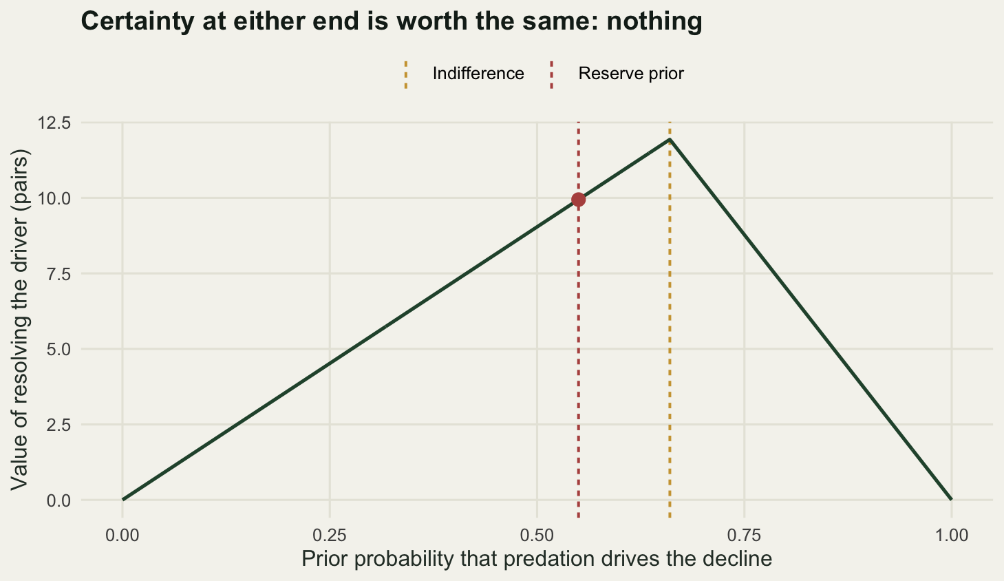
At a prior of 0.55 the value of resolving the driver is 9.9434 pairs. Push the prior up to the indifference point of 0.6601 and the value rises to 11.9342, its maximum, even though the reserve is now more confident about the driver than it was. Push it to certainty at either end and the value is zero. Confidence and value move in opposite directions over most of the right hand half of that curve, which is the practical content of the whole method.
Partial values, one unknown at a time
Perfect information about everything is not on sale. What is sometimes on sale is perfect information about one quantity. The expected value of partial perfect information asks what the decision is worth if one unknown is resolved and the others are left as they are: average, over the possible values of that one quantity, the best expected payoff computable once it is known.
evppi <- function(P, p, g) {
  base <- max(colSums(p * P))
  branches <- split(seq_along(p), g)
  sum(sapply(branches, function(i) max(colSums(p[i] * P[i, , drop = FALSE])))) - base
}

quantities <- c("cause", "lag", "rebound", "census")
ev_partial <- sapply(quantities, function(q) evppi(payoff, states$prob, states[[q]]))
print(round(ev_partial, 4))
cause lag rebound census
9.9434 1.7551 1.2579 0.0000 print(c(census_value_is_exactly_zero = identical(as.numeric(ev_partial["census"]), 0)))census_value_is_exactly_zero
TRUE print(rbind(rank_by_entropy = rank(-ent_prior), rank_by_value = rank(-ev_partial))) cause lag rebound census
rank_by_entropy 2 4 3 1
rank_by_value 1 2 3 4print(round(c(spearman_rank_correlation =
cor(ev_partial, ent_prior, method = "spearman"),
sum_of_partial_values = sum(ev_partial),
total_evpi = evpi_base,
overshoot = sum(ev_partial) - evpi_base), 4))spearman_rank_correlation sum_of_partial_values total_evpi
-0.4000 12.9565 10.2872
overshoot
2.6693 Resolving the driver is worth 9.9434 pairs. Resolving the restoration lag is worth 1.7551. Resolving the predator rebound is worth 1.2579. Resolving the census is worth zero, and again exactly zero, confirmed by identical rather than by rounding.
Set that against the entropies from the first chunk. The census is the most uncertain quantity in the problem at 1.0671 nats and it is worth nothing. The restoration lag is the least uncertain at 0.3669 nats and it is worth 1.7551 pairs, more than the predator rebound, which carries nearly twice its entropy. The Spearman rank correlation between the two orderings is -0.4. Ranking unknowns by how uncertain they are does not merely fail to reproduce the value ranking here; it gets the sign wrong.
The census is worth nothing for a structural reason, and the reason generalises. The current count multiplies every projected payoff by the same factor, so it scales all three alternatives together and cannot reorder them. Knowing it changes the forecast a great deal and changes the decision not at all. That is the most common shape of expensive irrelevance in conservation monitoring: a quantity everyone wants pinned down because it appears in the report, which enters the payoffs as a common factor.
The last two printed numbers are the ones that trip people up. The partial values sum to 12.9565 while the total expected value of perfect information is 10.2872, an overshoot of 2.6693 pairs. The partial values are not additive and they are not shares of a fixed pot. Resolving the driver alone already captures 9.9434 of a total of 10.2872, because the driver very nearly determines which alternative wins, and the lag and the rebound each recover value that the driver would have recovered too. Adding partial values is double counting. It can also fall the other way: two unknowns can be worth nothing separately and a great deal jointly, when the action depends on their combination rather than on either alone.
tempered <- function(p, t) { z <- p^t; z / sum(z) }

sweep_one <- function(q, lev, pr) {
  ts <- c(seq(0, 1, length.out = 21), exp(seq(log(1.05), log(40), length.out = 24)))
  do.call(rbind, lapply(ts, function(t) {
    pw <- tempered(pr, t)
    w <- states$prob / pr[match(states[[q]], lev)] * pw[match(states[[q]], lev)]
    data.frame(quantity = q, temper = t, ent = entropy(pw),
               value = evppi(payoff, w, states[[q]]))
  }))
}
sweep_tab <- rbind(sweep_one("cause", cause_lv, cause_pr),
                   sweep_one("lag", lag_lv, lag_pr),
                   sweep_one("rebound", reb_lv, reb_pr),
                   sweep_one("census", cen_lv, cen_pr))
flat <- sweep_tab[sweep_tab$temper == 0, ]
print(round(rbind(entropy_when_flat = flat$ent[match(quantities, flat$quantity)],
                  value_when_flat = flat$value[match(quantities, flat$quantity)],
                  largest_value_over_sweep =
                    tapply(sweep_tab$value, sweep_tab$quantity, max)[quantities]), 4))
cause lag rebound census
entropy_when_flat 0.6931 0.6931 0.6931 1.0986
value_when_flat 9.0395 4.3252 1.0483 0.0000
largest_value_over_sweep 11.8290 5.3807 1.8621 0.0000The sweep flattens or sharpens each prior in turn, holding the others fixed, by raising the prior to a power and renormalising. At a power of one it is the reserve’s own prior; at zero it is uniform, the most uncertain that quantity can be; at large powers it collapses onto its most likely value. That traces the value of each unknown across the full range of uncertainty it could have.
q_lab <- c(cause = "Driver of the decline", lag = "Restoration lag",
           rebound = "Predator rebound", census = "Current census")
sweep_tab$label <- factor(q_lab[sweep_tab$quantity], levels = q_lab)
at_prior <- sweep_tab[abs(sweep_tab$temper - 1) < 1e-9, ]

ggplot(sweep_tab, aes(ent, value, colour = label)) +
  geom_line(linewidth = 0.9) +
  geom_point(data = at_prior, size = 3.2) +
  scale_colour_manual(values = c(te_pal$forest, te_pal$clay,
                                 te_pal$gold, te_pal$green), name = NULL) +
  labs(x = "Entropy of the prior on that unknown (nats)",
       y = "Value of resolving it (pairs)",
       title = "More uncertainty does not mean more value") +
  theme_te() +
  theme(legend.position = "top")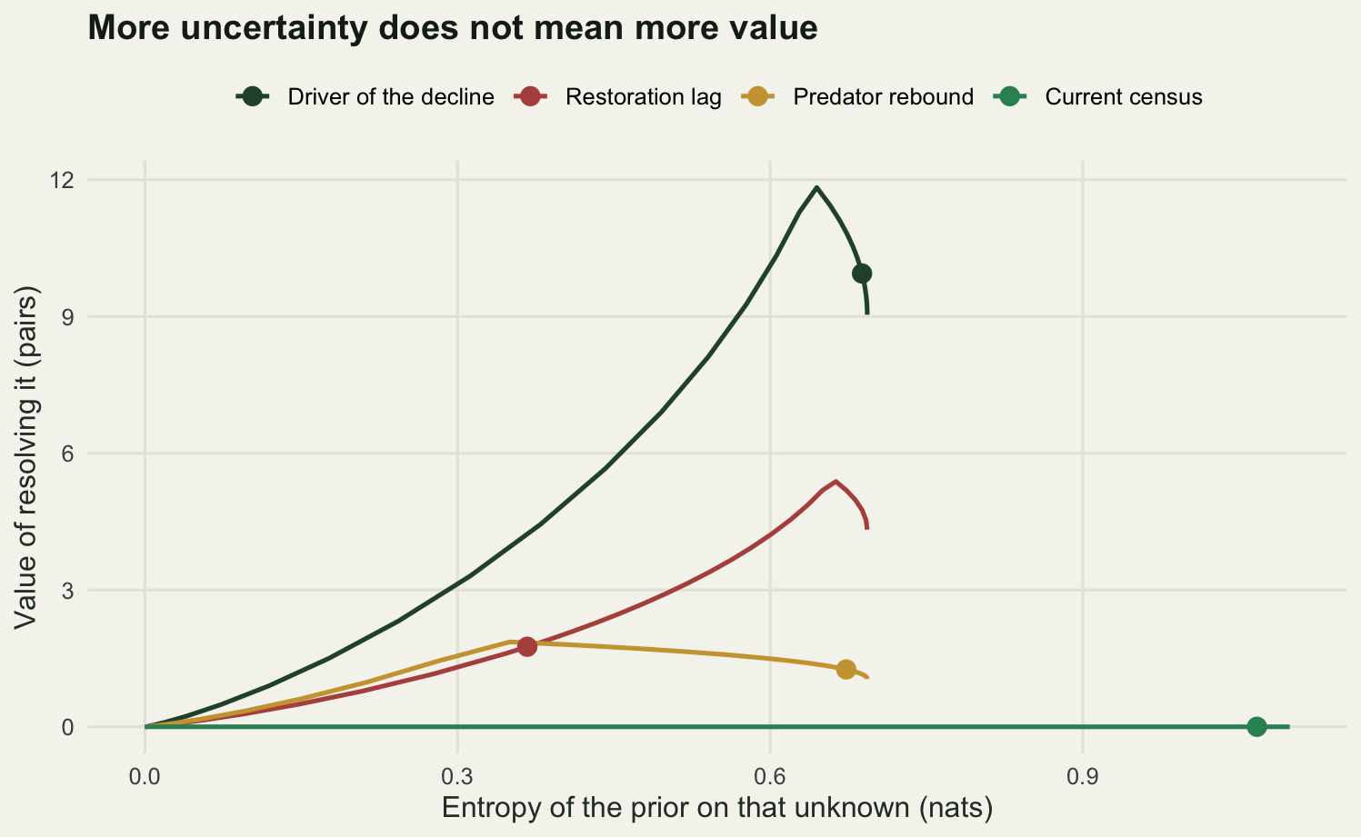
Flatten every prior to the most uncertain it can be and the values become 9.0395 pairs for the driver, 4.3252 for the restoration lag, 1.0483 for the predator rebound and zero for the census. The ordering by value survives that levelling, so it is a property of how each unknown enters the payoffs rather than of how much doubt happens to attach to it. The spacing does change: at equal uncertainty the restoration lag pulls well clear of the predator rebound, where at the reserve’s own priors the two sit close together.
None of the three paying curves has its maximum at maximum entropy. The largest value on the temper grid is 11.829 pairs for the driver, 5.3807 for the lag and 1.8621 for the rebound, and every one of those peaks belongs to a prior that is more confident than uniform, because the value is largest where the prior sits on the line at which the alternatives change places. The driver’s grid maximum falls a little short of the 11.9342 computed earlier for the same curve, because the grid steps from a temper of 3.1792 to one of 3.7244 and skips the 3.3080 that puts the prior exactly on the indifference point. The census curve is the one to take away. It is flat on zero from an entropy of 1.0986 all the way down to nothing, so no amount of doubt about the current population size, and no amount of resolving it, moves this decision by a single pair.
What an imperfect survey is worth
Perfect information is a bound, not an offer. A real study returns a noisy signal. Suppose the reserve can run a nest camera and predation survey that returns a verdict on the driver with a stated sensitivity and specificity, both equal to an accuracy that we will vary. The survey says “predation” or “habitat”, it is right with probability equal to that accuracy, and it is wrong otherwise.
The calculation has three steps and no new ideas. For each possible verdict, apply Bayes’ rule to get the posterior on the driver. Under that posterior, take the best alternative and its expected payoff. Average those over the probability of each verdict, and subtract the baseline. That is the expected value of sample information.
survey_cost <- 3

evsi <- function(q) {
  total <- 0
  for (k in 1:2) {
    lik <- if (k == 1) c(q, 1 - q) else c(1 - q, q)
    total <- total + max(colSums(cause_pr * lik * marginal))
  }
  total - max(colSums(cause_pr * marginal))
}

posterior_pred <- function(q) cause_pr[1] * q / (cause_pr[1] * q + cause_pr[2] * (1 - q))
q_star <- uniroot(function(q) posterior_pred(q) - p_star, c(0.5, 0.9999), tol = 1e-12)$root
q_break <- uniroot(function(q) evsi(q) - survey_cost, c(q_star, 1), tol = 1e-12)$root

acc <- c(0.50, 0.55, 0.60, q_star, 0.65, 0.70, q_break, 0.80, 0.90, 0.95, 0.99, 1.00)
print(round(cbind(accuracy = acc, evsi = sapply(acc, evsi),
                  net_of_cost = sapply(acc, evsi) - survey_cost), 4))
accuracy evsi net_of_cost
[1,] 0.5000 0.0000 -3.0000
[2,] 0.5500 0.0000 -3.0000
[3,] 0.6000 0.0000 -3.0000
[4,] 0.6138 0.0000 -3.0000
[5,] 0.6500 0.9330 -2.0670
[6,] 0.7000 2.2202 -0.7798
[7,] 0.7303 3.0000 0.0000
[8,] 0.8000 4.7946 1.7946
[9,] 0.9000 7.3690 4.3690
[10,] 0.9500 8.6562 5.6562
[11,] 0.9900 9.6860 6.6860
[12,] 1.0000 9.9434 6.9434print(round(c(indifference_probability = p_star,
threshold_accuracy = q_star,
posterior_at_threshold = posterior_pred(q_star),
evsi_at_perfect_accuracy = evsi(1),
partial_evpi_for_driver = as.numeric(ev_partial["cause"]),
driver_share_of_total_evpi =
100 * as.numeric(ev_partial["cause"]) / evpi_base), 4)) indifference_probability threshold_accuracy
0.6601 0.6138
posterior_at_threshold evsi_at_perfect_accuracy
0.6601 9.9434
partial_evpi_for_driver driver_share_of_total_evpi
9.9434 96.6588 print(round(c(survey_cost = survey_cost, break_even_accuracy = q_break,
evsi_at_break_even = evsi(q_break),
net_gain_at_accuracy_0.9 = evsi(0.90) - survey_cost), 4)) survey_cost break_even_accuracy evsi_at_break_even
3.0000 0.7303 3.0000
net_gain_at_accuracy_0.9
4.3690 acc_seq <- seq(0.5, 1, length.out = 401)
evsi_df <- data.frame(accuracy = acc_seq, value = sapply(acc_seq, evsi))
notes <- data.frame(accuracy = c(q_star, q_break),
value = c(0, survey_cost),
label = c("Never changes the action", "Breaks even"))
ggplot(evsi_df, aes(accuracy, value)) +
geom_hline(yintercept = evsi(1), colour = te_pal$sage,
linetype = "22", linewidth = 0.7) +
geom_hline(yintercept = survey_cost, colour = te_pal$clay, linewidth = 0.7) +
geom_line(colour = te_pal$forest, linewidth = 0.9) +
geom_point(data = notes, aes(shape = label), size = 3.4, colour = te_pal$ink) +
annotate("text", x = 0.505, y = evsi(1) - 0.55, hjust = 0, size = 3,
colour = te_pal$green, label = "Value of certainty about the driver") +
annotate("text", x = 0.505, y = survey_cost + 0.5, hjust = 0, size = 3,
colour = te_pal$clay, label = "Cost of the survey") +
scale_shape_manual(values = c("Never changes the action" = 1,
"Breaks even" = 16), name = NULL) +
labs(x = "Survey accuracy (sensitivity and specificity)",
y = "Value of the survey (pairs)",
title = "A survey is worth nothing until it can change the answer") +
theme_te() +
theme(legend.position = "top")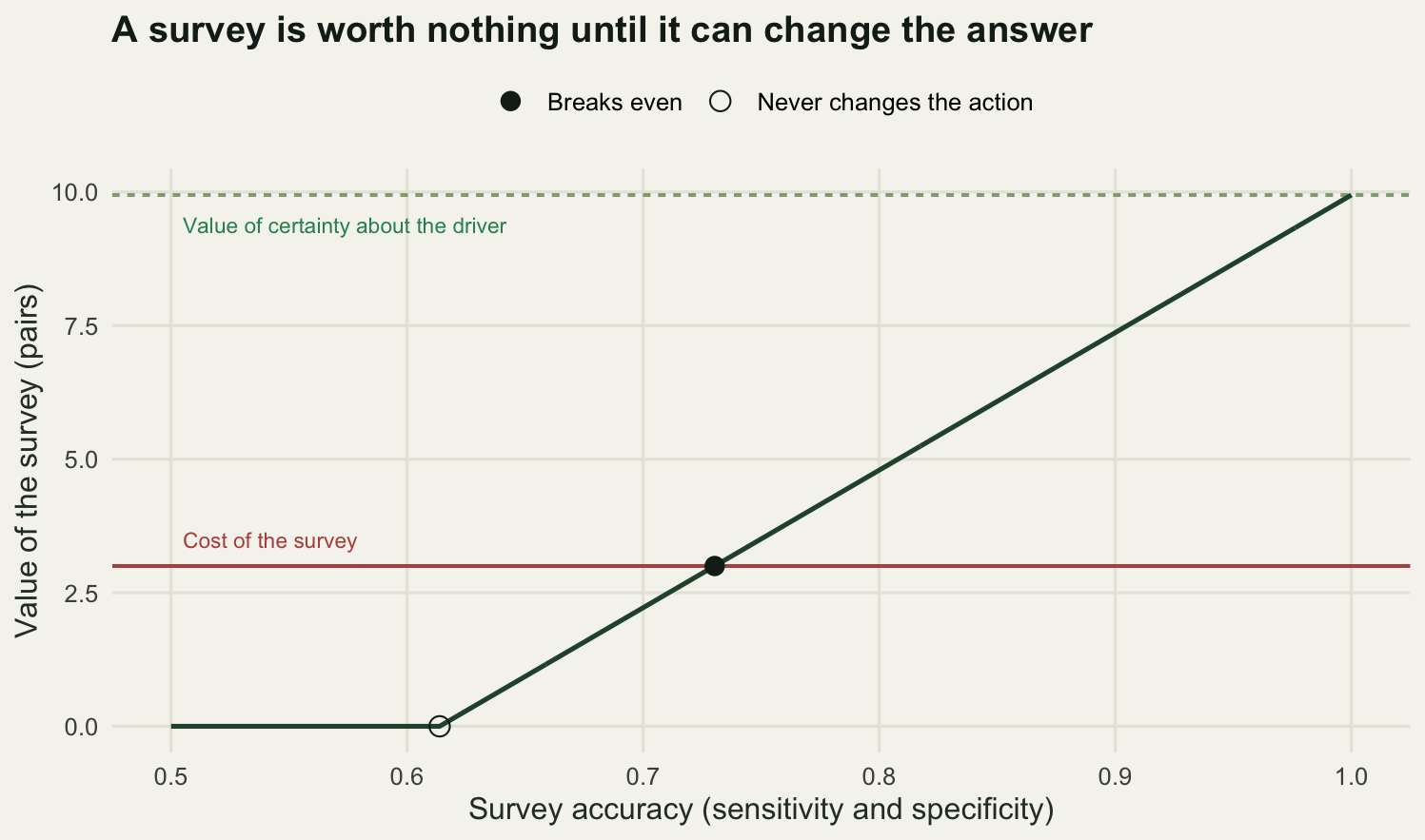
Three features of that line are worth stating separately.
It ends where it should. At an accuracy of one the survey is worth 9.9434 pairs, which is exactly the partial value of perfect information for the driver computed in the previous section. A survey that resolves one unknown perfectly cannot be worth more than perfect information about that unknown, and it is not worth the total expected value of perfect information either: the driver carries 96.6588 per cent of the total here, and the remaining value lives in unknowns this survey does not touch. The ceiling on a study is the partial value of what the study measures.
It starts flat. Up to an accuracy of 0.6138 the survey is worth zero, and it is worth zero at any price, including free. The reason is in the posterior arithmetic. The reserve starts at 0.55 on predation and restoration stays the better bet until that probability reaches 0.6601. A verdict of “predation” from a survey of accuracy 0.6138 lifts the posterior to exactly 0.6601, so anything weaker leaves the posterior short of the switch. Both verdicts then leave restoration best, the decision is the same whatever the survey says, and the survey is decoration.
It crosses the cost at a definite point. Price the survey at 3 pairs of projected population, which is the season of delay and the diverted budget converted into the currency of the decision. The break even accuracy is 0.7303. At an accuracy of 0.9 the survey nets 4.369 pairs after cost, so a good camera study is clearly worth running here; at 0.7 it returns 2.2202 against a cost of 3 and is a loss. The gap between 0.6138 and 0.7303 is the interesting band: those surveys do sometimes change the decision, and still should not be bought.
The honest limit: EVPI is conditional on the alternatives
Everything above is conditional on three alternatives. That conditioning is not a technicality, and it cuts in a direction most users do not expect.
The reserve costed a fourth option late in the process: fence and hydrologically manage a core compartment, so that inside the fence both drivers are handled at once. The compartment is small, so the benefit is capped, but it is the same benefit whatever the driver turns out to be. Add it to the set and recompute the baseline and the value of perfect information.
core_gain <- 0.030
payoff4 <- cbind(payoff, core = states$census * exp(horizon * (r_decline + core_gain)))
ev_prior4 <- colSums(states$prob * payoff4)
evpi4 <- evpi(payoff4, states$prob)

print(round(ev_prior4, 3))
monitor predator habitat core
70.336 90.322 96.179 110.308 print(round(c(evpi_three_alternatives = evpi_base, evpi_four_alternatives = evpi4,
fall_in_pairs = evpi_base - evpi4,
fall_percent = 100 * (1 - evpi4 / evpi_base),
baseline_three = max(ev_prior), baseline_four = max(ev_prior4),
evpi_percent_of_baseline_four = 100 * evpi4 / max(ev_prior4)), 3)) evpi_three_alternatives evpi_four_alternatives
10.287 3.669
fall_in_pairs fall_percent
6.618 64.336
baseline_three baseline_four
96.179 110.308
evpi_percent_of_baseline_four
3.326 print(table(best_in_state = apply(payoff4, 1, function(z) colnames(payoff4)[which.max(z)])))best_in_state
core habitat predator
12 6 6 The fenced core projects 110.308 pairs under the prior, beating restoration’s 96.179, so it takes over as the best action. The expected value of perfect information falls from 10.287 pairs to 3.669, a drop of 6.618 pairs or 64.336 per cent. As a fraction of the decision it falls from 10.696 per cent to 3.326 per cent.
Nothing was learned. No prior changed, no survey was run, no entropy moved. The value of knowing fell by two thirds because a new alternative was added that does moderately well whatever the state turns out to be. It is best in 12 of the 24 states and never far behind in the others, so knowing the state buys much less than it did.
That is the honest limit of the method, and it has a sharp practical edge. A low expected value of perfect information has two completely different causes and the arithmetic cannot tell them apart. Either the uncertainty genuinely does not matter, in which case act now and spend the research money elsewhere, or the alternative set is too narrow and too flat to exploit what you would learn. The second case looks identical on the printout. A decision analysis over three alternatives that all fail in the same states will report a small value of information and a large sense of reassurance, and the correct response is to go back and invent a better alternative rather than to declare the uncertainty unimportant.
The direction of the effect is worth holding on to, because it is counterintuitive in both readings. A better alternative reduces the value of information. A worse or more polarised alternative set inflates it. If you ever want a high expected value of information, the cheapest way to get one is to consider only extreme options, which is exactly the wrong reason to fund a study.
Two smaller limits sit alongside. Everything here assumes the payoff is the thing to maximise in expectation, so a manager who is risk averse over extinction rather than expectation over pairs is computing a different quantity and will get a different ranking of unknowns. And the priors are inputs, not measurements: the value of information is as arguable as the probabilities fed into it, which is why the sweep in the third figure matters more than any single number on it.
Where to go next
The natural sequel is the case where the decision repeats. If the reserve will choose again next year, a management action is itself an experiment, and the value of information becomes something you can earn by acting rather than only by surveying; adaptive management and learning sets that loop up and measures what the learning is worth. Before that, it is worth running the diagnostics on the analysis above, because a value of information calculation inherits every weakness of the payoff model underneath it.
References
Runge MC, Converse SJ, Lyons JE 2011 Biological Conservation 144(4):1214-1223 (10.1016/j.biocon.2010.12.020)
Canessa S, Guillera-Arroita G, Lahoz-Monfort JJ, Southwell DM, Armstrong DP, Chades I, Lacy RC, Converse SJ 2015 Methods in Ecology and Evolution 6(10):1219-1228 (10.1111/2041-210X.12423)
Maxwell SL, Rhodes JR, Runge MC, Possingham HP, Ng CF, McDonald-Madden E 2015 Journal of Applied Ecology 52(1):12-20 (10.1111/1365-2664.12373)
Raiffa H, Schlaifer R 1961 Applied Statistical Decision Theory. Division of Research, Graduate School of Business Administration, Harvard University (no DOI)