library(ggplot2)

te_pal <- list(forest = "#275139", green = "#2f8f63", sage = "#93a87f",
               clay = "#b5534e", gold = "#cda23f", line = "#dad9ca",
               ink = "#16241d", paper = "#f5f4ee")

theme_te <- function() {
  theme_minimal(base_size = 12) +
    theme(panel.grid.minor = element_blank(),
          panel.grid.major = element_line(colour = "#e7e6dc"),
          plot.background = element_rect(fill = "#f5f4ee", colour = NA),
          panel.background = element_rect(fill = "#f5f4ee", colour = NA),
          plot.title = element_text(face = "bold", colour = te_pal$ink),
          axis.title = element_text(colour = "#2c3a31"))
}Checking a decision analysis
R
conservation
decision analysis
model diagnostics
ecology tutorial
ggplot2
Four checks on a conservation decision analysis in R: weight and table sensitivity, the value of information, the alternative set, and the attitude to risk.
The three earlier posts in this cluster each end with something a manager can sign. Structured decision making in R builds a consequence table, screens it for dominance, normalises the columns and combines them with swing weights into one score per alternative. The expected value of information prices the uncertainty in that score: what perfect knowledge would be worth, which parameter carries the value, and what a survey of a given size would buy. Adaptive management and learning puts the same decision on a timeline, updates model weights from monitoring and compares passive learning with deliberate probing. Every one of them returns a ranked table, and every ranked table looks defensible on the page.
This post tries to break them. It is four checks run on a single conservation decision, built here so that the truth is known throughout: how far any one input has to move before the recommendation changes; whether the uncertainty in the analysis is the kind that could change the decision; what happens to the ranking when the set of alternatives is altered; and whether the answer survives a change of attitude to risk. The checks are cheap: a few lines of arithmetic on top of the analysis you already have, and none of them needs new data.
Nothing below is quoted from a rule of thumb. Every threshold and every comparison is measured on the same decision, and where a check comes back saying that the recommendation is weaker than it looked, that is the result and it stays in.
The decision under test
A lowland wet grassland reserve holds a declining population of a ground-nesting wader. The reserve has one budget and four candidate uses of it: fence the nesting compartment against mammalian predators, install and run sluices to hold water in the ditches through the breeding season, cut the encroaching scrub back to open sward, or spend nothing beyond the monitoring the designation already requires. Four objectives are on the table: the probability the population persists over the planning horizon, the annual cost in thousands of pounds, the area of suitable habitat delivered in hectares, and a local acceptance score out of ten. Cost is minimised and the other three are maximised.
Persistence comes from a stated model rather than from opinion. The population starts at 120 pairs, quasi-extinction is 20, environmental variation on the log scale has a standard deviation of 0.18, and the probability of avoiding quasi-extinction over the horizon is the diffusion first-passage expression: given a mean log growth rate and a starting distance above the threshold, the extinction probability has a closed form and persistence is one minus it. Each action adds an increment to the mean log growth rate, and the size of that increment depends on things nobody knows yet.
Those unknowns are eight dimensionless multipliers, each with a prior mean of exactly one and three levels. Predation pressure and fence reliability scale the fence’s demographic benefit; spring drought frequency and the water available to the sluices given upstream abstraction scale the water benefit; scrub regrowth erodes the benefit and the habitat gain of cutting; the baseline decline scales the growth rate of every alternative alike; local goodwill scales acceptance of the fence; and a maintenance multiplier moves the fence’s running cost. The full state space is the product of the eight, and the state probabilities are the products of the level probabilities.
The value model is the one from the first post. Each objective is normalised to a zero to one scale by the best and worst entries in the consequence table, and the normalised scores are combined with swing weights. Because the normalisation is linear and its endpoints are fixed by the table, the expected value of an alternative is exactly the value of its expected consequences, which is why the first check can be run on a four by four table rather than on the whole state space. That equality fails for the utility function in check 4 and for the maximum inside the value of information, and both are computed state by state.
q_lev <- list(predation = c(0.55, 1.00, 1.45),
              drought = c(0.70, 1.00, 1.30),
              inflow = c(0.35, 1.00, 1.65),
              regrowth = c(0.75, 1.00, 1.25),
              decline = c(0.70, 1.00, 1.30),
              reliability = c(0.85, 1.00, 1.15),
              goodwill = c(0.60, 1.00, 1.40),
              maintenance = c(0.20, 1.00, 1.80))
q_pr <- list(predation = c(0.30, 0.40, 0.30),
             drought = c(0.25, 0.50, 0.25),
             inflow = c(0.30, 0.40, 0.30),
             regrowth = c(0.30, 0.40, 0.30),
             decline = c(0.30, 0.40, 0.30),
             reliability = c(0.30, 0.40, 0.30),
             goodwill = c(0.25, 0.50, 0.25),
             maintenance = c(0.30, 0.40, 0.30))
q_name <- names(q_lev)

lev_idx <- expand.grid(lapply(q_lev, seq_along))
state <- as.data.frame(mapply(function(v, i) v[i], q_lev, lev_idx, SIMPLIFY = FALSE))
p_state <- Reduce(`*`, mapply(function(p, i) p[i], q_pr, lev_idx, SIMPLIFY = FALSE))
q_mean <- sapply(q_name, function(k) sum(q_pr[[k]] * q_lev[[k]]))
q_var <- sapply(q_name, function(k) sum(q_pr[[k]] * (q_lev[[k]] - q_mean[k])^2))

horizon <- 30; n_start <- 120; n_quasi <- 20; env_sd <- 0.18
d0 <- log(n_start / n_quasi)

persistence <- function(mu) {
  z1 <- (-d0 - mu * horizon) / (env_sd * sqrt(horizon))
  z2 <- (-d0 + mu * horizon) / (env_sd * sqrt(horizon))
  1 - pmin(pnorm(z1) + exp(-2 * mu * d0 / env_sd^2) * pnorm(z2), 1)
}
base_mu <- function(st) -0.045 * st$decline

acts <- list(
  "Predator fence" = function(st) cbind(
    persistence = persistence(base_mu(st) + 0.055 * st$predation * st$reliability),
    cost = 44 + 4 * st$maintenance, habitat = rep(26, nrow(st)),
    acceptance = 6.2 * st$goodwill),
  "Water control" = function(st) cbind(
    persistence = persistence(base_mu(st) + 0.040 * st$drought * st$inflow),
    cost = rep(41, nrow(st)), habitat = rep(38, nrow(st)),
    acceptance = rep(6.8, nrow(st))),
  "Scrub removal" = function(st) cbind(
    persistence = persistence(base_mu(st) + 0.022 / st$regrowth),
    cost = rep(22, nrow(st)), habitat = 20 / st$regrowth,
    acceptance = rep(8.0, nrow(st))),
  "Monitoring only" = function(st) cbind(
    persistence = persistence(base_mu(st)),
    cost = rep(7, nrow(st)), habitat = rep(4, nrow(st)),
    acceptance = rep(7.0, nrow(st))))

obj_dir <- c(persistence = 1, cost = -1, habitat = 1, acceptance = 1)
obj_name <- names(obj_dir)
w_base <- c(persistence = 0.46, cost = 0.16, habitat = 0.22, acceptance = 0.16)

cons_of <- function(a, st = state) lapply(a, function(f) f(st))
table_of <- function(cons, p = p_state) t(sapply(cons, function(m) colSums(m * p)))
norm_of <- function(tab) {
  lo <- apply(tab, 2, min); hi <- apply(tab, 2, max)
  for (j in seq_along(obj_dir))
    tab[, j] <- if (obj_dir[j] > 0) (tab[, j] - lo[j]) / (hi[j] - lo[j]) else
      (hi[j] - tab[, j]) / (hi[j] - lo[j])
  tab
}
ev_of <- function(tab, w = w_base) as.vector(norm_of(tab) %*% w)
win_of <- function(tab, w = w_base) which.max(ev_of(tab, w))
val_states <- function(cons, tab, w = w_base) {
  lo <- apply(tab, 2, min); hi <- apply(tab, 2, max)
  sapply(cons, function(m) {
    vv <- sapply(seq_along(obj_dir), function(j)
      if (obj_dir[j] > 0) (m[, j] - lo[j]) / (hi[j] - lo[j]) else
        (hi[j] - m[, j]) / (hi[j] - lo[j]))
    as.vector(vv %*% w)
  })
}
run <- function(a, w = w_base) {
  cons <- cons_of(a); tab <- table_of(cons); vs <- val_states(cons, tab, w)
  ev <- ev_of(tab, w); names(ev) <- names(a)
  list(cons = cons, tab = tab, v = vs, ev = ev, best = names(a)[which.max(ev)],
       evpi = sum(p_state * apply(vs, 1, max)) - max(ev))
}

alt_name <- names(acts)
b <- run(acts)
c(states = nrow(state), quantities = length(q_lev), alternatives = length(acts),
  horizon = horizon, start_size = n_start, quasi_extinction = n_quasi)
states quantities alternatives horizon
6561 8 4 30
start_size quasi_extinction
120 20 round(c(env_sd = env_sd, prior_means = mean(q_mean), w_base), 3) env_sd prior_means persistence cost habitat acceptance
0.18 1.00 0.46 0.16 0.22 0.16 print(round(b$tab, 3)) persistence cost habitat acceptance
Predator fence 0.930 48 26.0 6.2
Water control 0.861 41 38.0 6.8
Scrub removal 0.787 22 20.8 8.0
Monitoring only 0.565 7 4.0 7.0print(round(b$ev, 4)) Predator fence Water control Scrub removal Monitoring only
0.6024 0.6733 0.6499 0.2311 round(c(margin = diff(sort(b$ev, decreasing = TRUE)[2:1]),
spread = diff(range(b$ev))), 4)margin.Water control spread
0.0234 0.4422 Eight uncertain quantities at three levels each make 6561 states of nature. The consequence table is the prior mean of each alternative under each objective: the fence buys the highest persistence at 0.930 and costs 48 thousand a year, water control gives 0.861 for 41, scrub removal gives 0.787 for 22 and leads on acceptance at 8.0, and monitoring alone gives 0.565 for 7. With swing weights of 0.46 on persistence, 0.22 on habitat and 0.16 each on cost and acceptance, water control scores 0.6733, scrub removal 0.6499, the fence 0.6024 and monitoring 0.2311.
The recommendation is water control, by 0.0234 on a scale whose full spread from best to worst alternative is 0.4422. Written up, that is a decision analysis: a table, a weight set, a winner and a runner-up. Everything from here is an attempt to find out how much that winner is worth.
Check 1: how firm is the recommendation?
A recommendation is firm if it takes a large change in an input to overturn it. The problem is that the inputs live on different scales, so “a large change” has to be defined for each of them separately and then converted into something comparable. Three kinds of input go into the score: the weights, the entries of the consequence table, and the probabilities on the states of nature. For each, the check finds the smallest change to a single value that hands the recommendation to another alternative, and reports it as a percentage of that input’s own scale.
Weights live on the unit interval and must sum to one, so moving one weight means renormalising the others proportionally; the distance is then measured in percentage points of the weight scale. Table entries are shifted by adding a constant to one cell, which moves the whole distribution of that consequence and, if the cell is an endpoint, moves the normalisation too; the distance is measured against the range of that objective across alternatives. State probabilities are moved one marginal level at a time, with the remaining levels of that quantity renormalised; the distance is again in percentage points. Each search is a coarse scan followed by bisection on the boundary.
flip <- function(fun, x0, lo, hi, n = 600) {
  x0 <- unname(x0)
  xs <- sort(unique(c(seq(lo, hi, length.out = n), x0)))
  wn <- vapply(xs, fun, numeric(1)); w0 <- fun(x0)
  bad <- which(wn != w0)
  if (!length(bad)) return(c(dist = NA_real_, at = NA_real_, to = NA_real_))
  best <- Inf; at <- NA; to <- NA
  for (i in bad) {
    j <- if (xs[i] > x0) i - 1L else i + 1L
    if (j < 1L || j > length(xs) || wn[j] != w0) next
    a <- xs[j]; bb <- xs[i]
    for (it in 1:50) { m <- (a + bb) / 2; if (fun(m) == w0) a <- m else bb <- m }
    if (abs(bb - x0) < best) { best <- abs(bb - x0); at <- bb; to <- fun(bb) }
  }
  c(dist = unname(best), at = unname(at), to = unname(to))
}

w_move <- function(t, j) { w <- w_base * (1 - t) / (1 - w_base[j]); w[j] <- t; w }
w_flip <- t(sapply(seq_along(w_base), function(j)
  flip(function(t) win_of(b$tab, w_move(t, j)), w_base[j], 0, 1)))
rownames(w_flip) <- obj_name
print(round(cbind(w_flip[, c("dist", "at")], pct = 100 * w_flip[, "dist"],
                  to = w_flip[, "to"]), 4))
dist at pct to
persistence 0.0707 0.3893 7.0700 3
cost 0.0403 0.2003 4.0344 3
habitat 0.0378 0.1822 3.7795 3
acceptance 0.0285 0.1885 2.8461 3rng <- apply(b$tab, 2, function(x) diff(range(x)))
ent_flip <- do.call(rbind, lapply(seq_along(alt_name), function(i)
do.call(rbind, lapply(seq_along(obj_name), function(j) {
z <- flip(function(d) { tb <- b$tab; tb[i, j] <- tb[i, j] + d; win_of(tb) },
0, -1.5 * rng[j], 1.5 * rng[j])
data.frame(alternative = alt_name[i], objective = obj_name[j],
shift = unname(z["dist"]), pct = unname(100 * z["dist"] / rng[j]))
}))))
print(head(ent_flip[order(ent_flip$pct), ], 4), row.names = FALSE) alternative objective shift pct
Scrub removal persistence 0.01855606 5.08259
Water control persistence 0.01855606 5.08259
Scrub removal habitat 3.61325940 10.62723
Scrub removal cost 5.99110290 14.61245cond_pair <- function(k, l) {
sel <- lev_idx[[k]] == l
pin <- p_state[sel] / sum(p_state[sel]); pout <- p_state[!sel] / sum(p_state[!sel])
list(inside = t(sapply(b$cons, function(m) colSums(m[sel, ] * pin))),
outside = t(sapply(b$cons, function(m) colSums(m[!sel, ] * pout))))
}
prob_flip <- do.call(rbind, lapply(q_name, function(k)
do.call(rbind, lapply(seq_along(q_lev[[k]]), function(l) {
ct <- cond_pair(k, l)
z <- flip(function(t) win_of(t * ct$inside + (1 - t) * ct$outside),
q_pr[[k]][l], 0, 1)
data.frame(quantity = k, level = l, prior = q_pr[[k]][l],
shift = unname(z["dist"]), pct = unname(100 * z["dist"]))
}))))
print(head(prob_flip[order(prob_flip$pct), ], 4), row.names = FALSE) quantity level prior shift pct
inflow 1 0.30 0.0861516 8.61516
goodwill 1 0.25 0.0978647 9.78647
goodwill 3 0.25 0.0978647 9.78647
inflow 3 0.30 0.1206714 12.06714round(c(weight_pct = min(100 * w_flip[, "dist"]),
entry_pct = min(ent_flip$pct, na.rm = TRUE),
probability_pct = min(prob_flip$pct, na.rm = TRUE)), 3) weight_pct entry_pct probability_pct
2.846 5.083 8.615 alt_col <- c("Predator fence" = te_pal$clay, "Water control" = te_pal$forest,
"Scrub removal" = te_pal$gold, "Monitoring only" = te_pal$sage)
w_curve <- do.call(rbind, lapply(seq_along(w_base), function(j) {
tt <- seq(0, 1, by = 0.004)
ee <- t(sapply(tt, function(t) ev_of(b$tab, w_move(t, j))))
data.frame(objective = obj_name[j], weight = rep(tt, length(alt_name)),
ev = as.vector(ee), alternative = rep(alt_name, each = length(tt)))
}))
w_curve$objective <- factor(w_curve$objective, levels = obj_name)
w_curve$alternative <- factor(w_curve$alternative, levels = alt_name)
w_mark <- data.frame(objective = factor(obj_name, levels = obj_name),
weight = as.numeric(w_base))
ggplot(w_curve, aes(weight, ev, colour = alternative)) +
geom_vline(data = w_mark, aes(xintercept = weight), colour = te_pal$ink,
linetype = "22", linewidth = 0.5) +
geom_line(linewidth = 0.8) +
facet_wrap(~objective) +
scale_colour_manual(values = alt_col, name = NULL) +
labs(x = "Weight on that objective", y = "Expected value",
title = "How far a single weight has to move") +
theme_te() +
theme(legend.position = "top",
strip.text = element_text(colour = te_pal$ink, face = "bold"))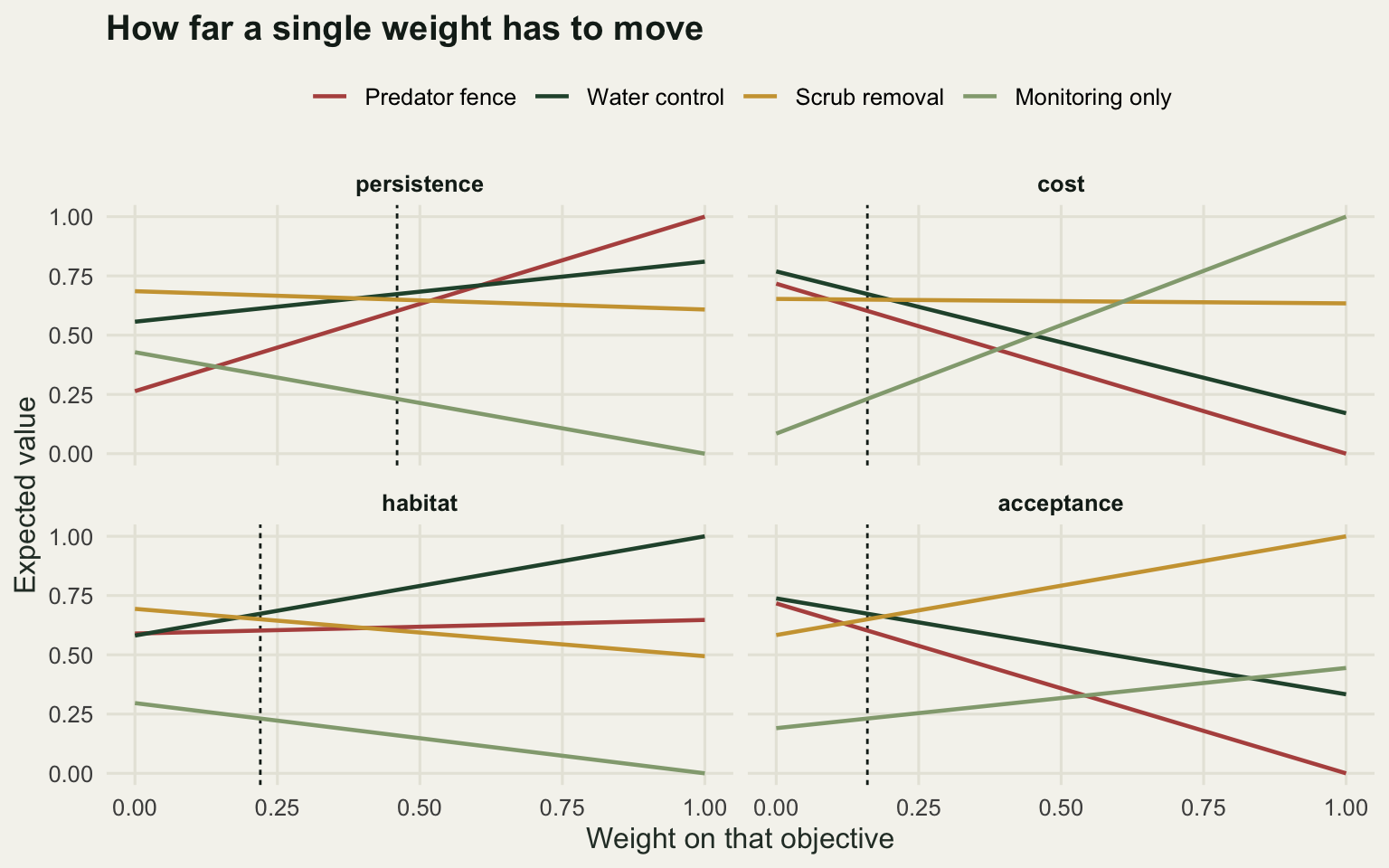
The three distances are 2.846 per cent for the weights, 5.083 per cent for the table and 8.615 per cent for the state probabilities, so the recommendation is most fragile to the weights, and by roughly a factor of three against the probabilities. The specific move is small: raising the weight on acceptance from 0.16 to 0.1885, with the other three shrinking in proportion, hands the decision to scrub removal. That is less than three percentage points on a quantity that came out of an elicitation exercise, and there is no data in the world that would settle it.
The table result is nearly as soft, and the arithmetic behind it is worth doing by hand. The gap between water control and scrub removal is 0.0234 of value. Persistence carries a weight of 0.46 over a range of 0.930 minus 0.565, so one unit of persistence is worth 0.46 divided by that range. Closing a gap of 0.0234 therefore takes a persistence shift of 0.01855606, or 5.083 per cent of the persistence range, and it does not matter whether you take it off water control or add it to scrub removal, which is why both appear with identical distances. A persistence estimate from a population model is not accurate to five per cent.
The probabilities are the sturdiest input, which is the reverse of the usual worry. The tightest of them is the probability on the low level of the water supply multiplier, which has to move 8.615 percentage points from its prior of 0.30 before the winner changes. Goodwill needs 9.78647 points and the rest need more.
set.seed(4071)
n_draw <- 20000
dir_w <- matrix(rexp(n_draw * length(w_base)), ncol = length(w_base))
dir_w <- dir_w / rowSums(dir_w)
simplex <- table(factor(alt_name[max.col(dir_w %*% t(norm_of(b$tab)))],
                        levels = alt_name)) / n_draw
c(weight_draws = n_draw)
weight_draws
20000 print(round(simplex, 4))
 Predator fence   Water control   Scrub removal Monitoring only
         0.0544          0.2806          0.6034          0.0616
The one-at-a-time sweep understates the problem, because weights move together. Drawing 20000 weight vectors uniformly from the simplex and recording which alternative wins each time gives a blunter number: water control, the recommendation, wins in 0.2806 of the weight simplex, while scrub removal wins in 0.6034 of it. The fence takes 0.0544 and monitoring 0.0616. The recommended alternative is a minority winner over the space of possible preferences, and it holds its position only because the elicited weights sit inside the region where it does win. That is not an argument against the analysis. It is an argument for reporting the region, because the analysis is now carrying the weights rather than the evidence.
Check 2: is the uncertainty decision-relevant?
The expected value of perfect information is the gap between what could be achieved by choosing the best alternative in each state of nature and what is achieved by choosing one alternative for all of them. It is the ceiling on what any study, survey or trial could contribute, and it is computed on the same value scale as the score itself. The partial version conditions on one uncertain quantity at a time: learn that quantity exactly, choose the best alternative given that knowledge alone, and see how much better off you are.
pevpi <- sapply(q_name, function(k)
  sum(sapply(seq_along(q_lev[[k]]), function(l) {
    sel <- lev_idx[[k]] == l
    max(as.vector(t(b$v[sel, ]) %*% p_state[sel]))
  })) - max(b$ev))
voi <- data.frame(quantity = q_name, variance = q_var, pevpi = pevpi)
print(round(voi[order(-voi$variance), 2:3], 4))
variance pevpi
maintenance 0.3840 0.0000
inflow 0.2535 0.0500
predation 0.1215 0.0009
goodwill 0.0800 0.0374
decline 0.0540 0.0061
drought 0.0450 0.0102
regrowth 0.0375 0.0233
reliability 0.0135 0.0000round(c(evpi = b$evpi, evpi_share_of_spread = b$evpi / diff(range(b$ev)),
pearson = cor(q_var, pevpi), spearman = cor(q_var, pevpi, method = "spearman"),
pevpi_sum = sum(pevpi)), 4) evpi evpi_share_of_spread pearson
0.0901 0.2037 0.0945
spearman pevpi_sum
0.1667 0.1279 print(round(table(factor(alt_name[max.col(b$v)], levels = alt_name)) / nrow(b$v), 3))
 Predator fence   Water control   Scrub removal Monitoring only
0.316 0.393 0.290 0.000 round(c(fence_behind_recommendation = unname(b$ev[2] - b$ev[1])), 4)fence_behind_recommendation
0.071 voi$label <- voi$quantity
ggplot(voi, aes(variance, pevpi)) +
geom_hline(yintercept = 0, colour = te_pal$line, linewidth = 0.8) +
geom_point(colour = te_pal$forest, size = 3) +
geom_text(aes(label = label), colour = te_pal$ink, size = 3.4, vjust = -0.9) +
scale_x_log10(expand = expansion(mult = c(0.1, 0.14))) +
coord_cartesian(ylim = c(-0.006, 0.062)) +
labs(x = "Prior variance of the multiplier",
y = "Partial expected value of perfect information",
title = "Spread and value are different things") +
theme_te()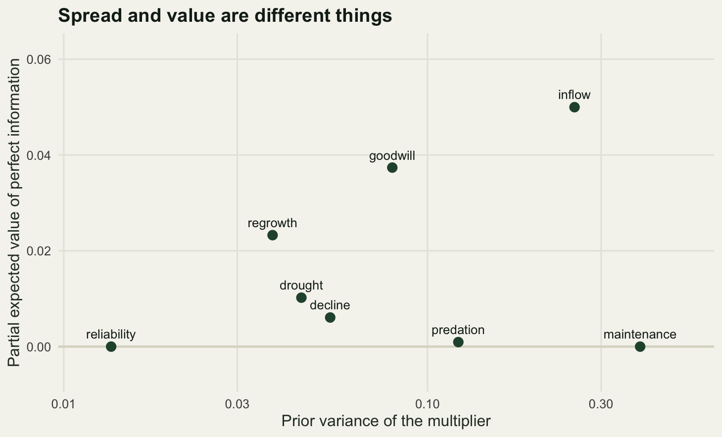
The whole decision has an expected value of perfect information of 0.0901, which is 0.2037 of the distance between the best and the worst alternative. That is a large number for a decision whose recommendation looked settled: a fifth of everything at stake is currently being decided by a coin that has not been tossed. The reason is visible in the winner shares printed in the block, where water control is the best choice in only 0.393 of states, the fence in 0.316 and scrub removal in 0.290. Monitoring alone is never the best choice in any state, which is the one genuinely reassuring result in this post.
Now the ordering. The maintenance multiplier has the largest prior variance of all eight, 0.3840, and a partial expected value of perfect information of 0.0000. Predation pressure has the third largest variance, 0.1215, and is worth 0.0009. Meanwhile scrub regrowth has a variance of 0.0375, a tenth of the maintenance multiplier’s, and is worth 0.0233, and goodwill with a variance of 0.0800 is worth 0.0374. Across the eight quantities the correlation between prior variance and partial value is 0.0945, and on ranks 0.1667. There is no relationship.
The mechanism is not subtle once it is stated. Prior variance is a property of one input on its own scale. Value of information is a property of the whole decision: a quantity is worth learning only if knowing it would make you act differently, and that depends on the coefficient the quantity enters with, on whether it separates two alternatives that are close, and on whether those alternatives are contenders at all. The maintenance multiplier swings the fence’s running cost by a few thousand pounds either way; that is real money and it is genuinely uncertain, but the fence is 0.071 of value behind the recommendation and no plausible maintenance bill closes that. Predation pressure is worth more in principle, since it drives the fence’s whole benefit, but again the fence is too far back for it to matter. The quantity that does pay is the water supply, at 0.0500, because it decides whether the recommended alternative works at all.
One arithmetic warning. The eight partial values sum to 0.1279, which is more than the total of 0.0901. Partial expected values of information do not add up, because two quantities can each be worth resolving on their own by pointing at the same switch. Anyone building a monitoring budget by summing the per-parameter values will buy too much information.
Check 3: the alternative set
The first two checks take the alternatives as given. This one does not, because the alternative set is an input like any other, and it enters the analysis twice: once through what is available to choose, and once through the endpoints that normalise every column of the table.
The first half of the check is constructive. Build a hybrid by combining two existing alternatives, holding water in the ditches and cutting the scrub in the same year, with the persistence benefits combined at a discount for overlap and the costs added at a small saving. Then ask three questions: does it dominate anything, does it win, and what does it do to the value of information?
hyb <- c(acts, list("Water and scrub" = function(st) cbind(
  persistence = persistence(base_mu(st) + 0.040 * st$drought * st$inflow +
                              0.6 * 0.022 / st$regrowth),
  cost = rep(58, nrow(st)), habitat = 38 + 0.7 * 20 / st$regrowth,
  acceptance = rep(7.4, nrow(st)))))
dud <- c(acts, list("Captive breeding" = function(st) cbind(
  persistence = persistence(base_mu(st) + 0.012),
  cost = rep(205, nrow(st)), habitat = rep(2, nrow(st)),
  acceptance = rep(4.5, nrow(st)))))
h <- run(hyb); d <- run(dud)
dominates <- function(tab, i, j) {
  g <- obj_dir * (tab[i, ] - tab[j, ])
  all(g >= 0) && any(g > 0)
}
print(round(h$tab[5, ], 3))
persistence cost habitat acceptance
0.922 58.000 52.560 7.400 print(round(h$ev, 4)) Predator fence Water control Scrub removal Monitoring only Water and scrub
0.5910 0.6334 0.6288 0.2311 0.7759 print(sapply(1:4, function(i) dominates(h$tab, 5, i)))[1] FALSE FALSE FALSE FALSEprint(sapply(1:4, function(i) dominates(d$tab, i, 5)))[1] TRUE TRUE TRUE FALSEround(c(evpi_base = b$evpi, evpi_hybrid = h$evpi, evpi_dud = d$evpi), 4) evpi_base evpi_hybrid evpi_dud
0.0901 0.0215 0.0701 The hybrid delivers a persistence of 0.922 and 52.56 hectares for 58 thousand a year, and it scores 0.7759, which is a long way clear of everything else. It dominates nothing at all: all four comparisons come back false, because it costs more than any of its parents and the cost objective blocks every dominance relation. That is the first result worth carrying away. In a table that contains a cost objective, dominance screening is close to powerless, since almost every action buys its benefit with money and is therefore worse on one column by construction. A screen that never fires is not evidence that the alternatives are all sensible.
The effect on the value of information is the sharper result. Adding the hybrid drops the expected value of perfect information from 0.0901 to 0.0215. Nothing was learned. The uncertainty is identical, the priors are identical, and the state space is identical. What changed is that the new alternative is good in most states at once, so the cost of committing before the uncertainty resolves has largely gone. Value of information is a property of the alternative set, not of the uncertainty, and a hedged alternative destroys most of it. That also means an expected value of perfect information calculation is not a measure of how much you do not know. It is a measure of how much your current options force you to gamble.
Now the sharper test, and the reason this check exists. Add an alternative nobody would choose: a captive breeding programme costing 205 thousand a year, delivering 2 hectares, a persistence of 0.692 and an acceptance of 4.5. It is dominated by three of the four existing alternatives, it scores 0.1591 in the extended table, and it will obviously never be picked. Adding it should change nothing about the others.
dud2 <- dud
dud2[[5]] <- function(st) cbind(
  persistence = persistence(base_mu(st) + 0.012),
  cost = rep(205, nrow(st)), habitat = rep(2, nrow(st)),
  acceptance = rep(9.0, nrow(st)))
d2 <- run(dud2)
print(round(rbind(dominated = d$tab[5, ], undominated = d2$tab[5, ]), 3))
persistence cost habitat acceptance
dominated 0.692 205 2 4.5
undominated 0.692 205 2 9.0print(round(d$ev, 4)) Predator fence Water control Scrub removal Monitoring only
0.8112 0.8303 0.7025 0.2865
Captive breeding
0.1591 print(sapply(1:4, function(i) dominates(d2$tab, i, 5)))[1] FALSE FALSE FALSE FALSEprint(round(d2$ev, 4)) Predator fence Water control Scrub removal Monitoring only
0.7335 0.7595 0.6454 0.2179
Captive breeding
0.3191 rk <- rbind(base = rank(-b$ev), with_dud = rank(-d$ev[1:4]),
with_undominated_dud = rank(-d2$ev[1:4]))
print(rk) Predator fence Water control Scrub removal Monitoring only
base 3 1 2 4
with_dud 2 1 3 4
with_undominated_dud 2 1 3 4round(c(rank_changes = sum(rk[1, ] != rk[2, ]),
cost_range_base = diff(range(b$tab[, "cost"])),
cost_range_dud = diff(range(d$tab[, "cost"])),
acceptance_range_base = diff(range(b$tab[, "acceptance"])),
acceptance_range_dud = diff(range(d$tab[, "acceptance"]))), 3) rank_changes cost_range_base cost_range_dud
2.0 41.0 198.0
acceptance_range_base acceptance_range_dud
1.8 3.5 set_lab <- c("Table as it stands", "Plus the hybrid", "Plus captive breeding")
cmp <- rbind(
data.frame(alternative = alt_name, ev = b$ev, set = set_lab[1]),
data.frame(alternative = alt_name, ev = h$ev[1:4], set = set_lab[2]),
data.frame(alternative = alt_name, ev = d$ev[1:4], set = set_lab[3]))
cmp$set <- factor(cmp$set, levels = set_lab)
cmp$alternative <- factor(cmp$alternative, levels = rev(alt_name))
row_lab <- levels(cmp$alternative)
cmp$ypos <- as.numeric(cmp$alternative) + c(0.17, 0, -0.17)[as.integer(cmp$set)]
span <- data.frame(row = seq_along(row_lab),
lo = as.numeric(tapply(cmp$ev, cmp$alternative, min)),
hi = as.numeric(tapply(cmp$ev, cmp$alternative, max)))
ggplot(cmp, aes(ev, ypos)) +
geom_segment(data = span, aes(x = lo, xend = hi, y = row, yend = row),
inherit.aes = FALSE, colour = te_pal$line, linewidth = 1.6) +
geom_point(aes(colour = set), size = 3.2) +
scale_y_continuous(breaks = seq_along(row_lab), labels = row_lab,
limits = c(0.5, length(row_lab) + 0.5)) +
scale_colour_manual(values = c(te_pal$forest, te_pal$green, te_pal$clay), name = NULL) +
labs(x = "Expected value", y = NULL,
title = "An option nobody would choose reorders the rest") +
theme_te() +
theme(legend.position = "top")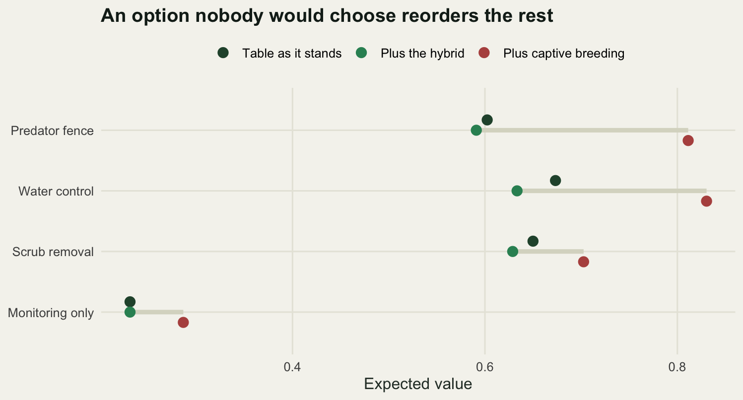
It changes the ranking. In the original table the order is water control, scrub removal, predator fence, monitoring. With captive breeding in the table the order is water control, predator fence, scrub removal, monitoring: two of the four ranks change, and the runner-up that a report would name as the fallback option is now a different action. Nobody’s beliefs changed, nobody’s preferences changed, and the added option is worthless.
The mechanism is the normalisation. The cost range across the alternatives goes from 41 to 198 when the expensive option joins, so every cost difference among the original four is compressed by almost a factor of five and the cost objective effectively drops out. The acceptance range goes from 1.8 to 3.5, halving the value of scrub removal’s lead on that column. Scrub removal was winning its second place on cheapness and popularity, and both of those advantages were shrunk by an alternative that will never be chosen. This is the classic rank reversal of additive value models with data-dependent scaling, and it is quiet: the winner survived here, so a reader checking only the top line would see nothing.
The obvious defence is the dominance screen, and here it would work, since captive breeding as specified is dominated. So the last block also runs a version whose acceptance score is 9.0, which makes it the best alternative on one column and therefore undominated by anything. It is still absurd: 205 thousand pounds a year for 2 hectares and a persistence of 0.692. It passes the screen, and it produces exactly the same reordering. The fix is not a better screen, it is to fix the ends of each value scale on externally defined best and worst levels, chosen before the alternatives are written down, rather than on the contents of the table.
Check 4: risk attitude
The score so far is an expectation, which is the right criterion only for a decision maker who is indifferent between a certain outcome and a gamble with the same mean. Conservation decisions are usually not taken that way. The check is to re-rank the alternatives under a concave utility function, and then under a downside criterion, and see whether the recommendation survives either.
The utility is the constant absolute risk aversion form applied to the overall value, and the certainty equivalent maps the expected utility back to the value scale so the alternatives stay comparable. The downside criterion states a minimum acceptable value and reports the probability of falling below it, which the decision maker then minimises.
util <- function(v, a) if (a == 0) v else (1 - exp(-a * v)) / a
cert <- function(eu, a) if (a == 0) eu else -log(1 - a * eu) / a
eu_of <- function(a) as.vector(t(util(b$v, a)) %*% p_state)
eu_win <- function(a) which.max(eu_of(a))
a_stated <- 5
a_flip <- flip(eu_win, 0, 0, 40, n = 400)
print(round(setNames(cert(eu_of(a_stated), a_stated), alt_name), 4))
Predator fence Water control Scrub removal Monitoring only
0.5162 0.5941 0.6062 0.1785 c(stated_coefficient = a_stated)stated_coefficient
5 round(c(a_switch = unname(a_flip["dist"])), 3)a_switch
3.598 cat("switches to:", alt_name[a_flip["to"]], "\n")switches to: Scrub removal print(round(sqrt(colSums(p_state * (b$v - rep(b$ev, each = nrow(b$v)))^2)), 4)) Predator fence Water control Scrub removal Monitoring only
0.1829 0.1607 0.1298 0.1484 v_min <- 0.55
short <- function(thr) sapply(seq_along(alt_name), function(i)
sum(p_state[b$v[, i] < thr]))
print(round(setNames(short(v_min), alt_name), 4)) Predator fence Water control Scrub removal Monitoring only
0.3743 0.2400 0.2100 1.0000 thr_grid <- seq(0.30, 0.85, by = 0.005)
short_tab <- t(sapply(thr_grid, short))
colnames(short_tab) <- alt_name
thr_win <- alt_name[apply(short_tab, 1, which.min)]
gamble <- c(gamble_low = 0.40, gamble_high = 0.80)
round(c(gamble, indifference = unname(cert(mean(util(gamble, a_flip["dist"])),
unname(a_flip["dist"])))), 4) gamble_low gamble_high indifference
0.4000 0.8000 0.5335 round(c(minimum_acceptable = v_min, threshold_low = min(thr_grid),
threshold_high = max(thr_grid),
distinct_winners_over_threshold = length(unique(thr_win)),
switches = sum(thr_win[-1] != thr_win[-length(thr_win)])), 3) minimum_acceptable threshold_low
0.55 0.30
threshold_high distinct_winners_over_threshold
0.85 3.00
switches
6.00 three <- c(ev = b$best, utility = alt_name[eu_win(a_stated)],
downside = alt_name[which.min(short(v_min))])
print(three) ev utility downside
"Water control" "Scrub removal" "Scrub removal" c(distinct_winners = length(unique(three)))distinct_winners
2 library(grid)
a_seq <- seq(0, 12, by = 0.1)
ce_long <- do.call(rbind, lapply(a_seq, function(a)
data.frame(a = a, ce = cert(eu_of(a), a), alternative = alt_name)))
ce_long$alternative <- factor(ce_long$alternative, levels = alt_name)
short_long <- do.call(rbind, lapply(seq_along(alt_name), function(i)
data.frame(thr = thr_grid, p = short_tab[, i], alternative = alt_name[i])))
short_long$alternative <- factor(short_long$alternative, levels = alt_name)
p_left <- ggplot(ce_long, aes(a, ce, colour = alternative)) +
geom_vline(xintercept = a_flip["dist"], colour = te_pal$ink,
linetype = "22", linewidth = 0.5) +
geom_line(linewidth = 0.8) +
scale_colour_manual(values = alt_col, name = NULL) +
guides(colour = guide_legend(nrow = 2)) +
labs(x = "Coefficient of absolute risk aversion", y = "Certainty equivalent",
title = "Risk aversion moves the winner") +
theme_te() + theme(legend.position = "top")
p_right <- ggplot(short_long, aes(thr, p, colour = alternative)) +
geom_vline(xintercept = v_min, colour = te_pal$ink,
linetype = "22", linewidth = 0.5) +
geom_step(linewidth = 0.8) +
scale_colour_manual(values = alt_col, name = NULL) +
guides(colour = guide_legend(nrow = 2)) +
labs(x = "Minimum acceptable value", y = "Probability of falling short",
title = "The downside criterion is not stable") +
theme_te() + theme(legend.position = "top")
grid.newpage()
pushViewport(viewport(layout = grid.layout(1, 2)))
print(p_left, vp = viewport(layout.pos.row = 1, layout.pos.col = 1))
print(p_right, vp = viewport(layout.pos.row = 1, layout.pos.col = 2))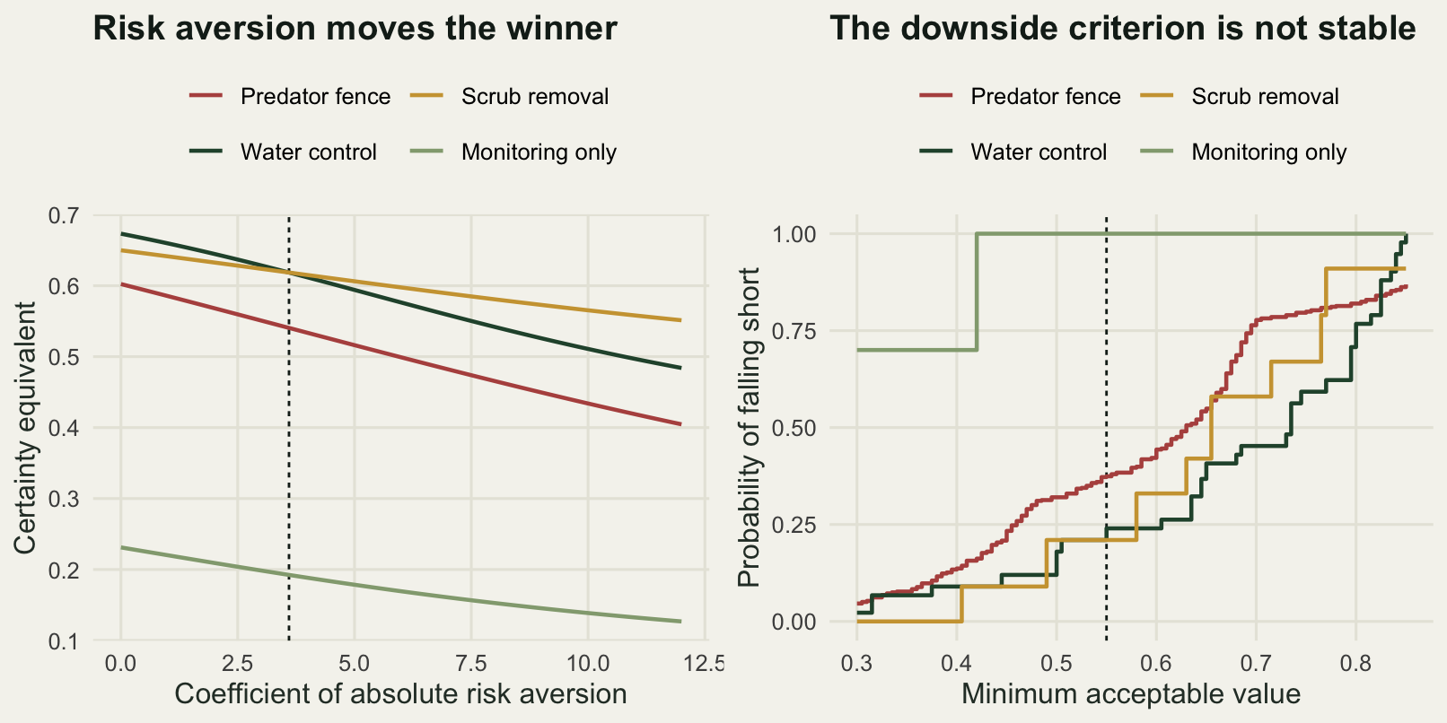
Ranking by expected value gives water control. Ranking by expected utility at a coefficient of 5 gives scrub removal, whose certainty equivalent is 0.6062 against 0.5941 for water control and 0.5162 for the fence. The switch happens at a coefficient of 3.598, and the reason is in the standard deviations printed below it: water control’s value has a standard deviation of 0.1607 across states while scrub removal’s is 0.1298, so water control is paying for its higher mean with more spread, and a moderately risk averse decision maker declines the trade. A coefficient of 3.598 on a value scale that runs from zero to one is not an extreme preference; it is roughly the attitude of someone who would swap a fifty-fifty gamble between 0.4 and 0.8 for a certain 0.5335.
The downside criterion agrees with the utility, and for a different reason. At a minimum acceptable value of 0.55, water control falls short in 0.2400 of states and scrub removal in 0.2100, so scrub removal wins again. Across the three criteria there are 2 distinct winners: the expected value recommendation stands alone, and the two risk sensitive criteria both prefer the runner-up.
The right hand panel carries a warning about the downside criterion itself. Sweeping the minimum acceptable value from 0.30 to 0.85 produces 3 distinct winners and 6 changes of hands. The criterion is a step function of a threshold that nobody has any principled way to set, and it throws away everything about how far short the shortfall is. It is useful as a second opinion and it is dangerous as a decision rule. Part of the raggedness here is the discrete state space, since with 6561 states the probability moves in jumps, but the instability is real and would survive a continuous prior.
What none of these checks can see
Every check above is a check of internal consistency. Check 1 asks whether the arithmetic is stable given the inputs. Check 2 asks what the stated uncertainty is worth given the alternatives. Check 3 asks whether the alternative set distorts the scales. Check 4 asks whether the aggregation rule is the right one. Not one of them asks whether the objectives are the objectives that matter, or whether the four alternatives include the good one.
That second gap can be measured rather than merely asserted. The uncertainty with the highest partial value in check 2 was the water available to the sluices, which depends on an abstraction licence held upstream. Every alternative on the table treats that licence as a fact of the world. Suppose instead that the licence can be bought out and the natural inflow restored: a one off cost amortised at 36 thousand a year, a demographic benefit that does not depend on the supply multiplier because the supply is no longer in question, 46 hectares of wet habitat, and an acceptance of 6.6 because the neighbours are not all pleased.
out <- c(acts, list("Abstraction buy-out" = function(st) cbind(
  persistence = persistence(base_mu(st) + 0.050),
  cost = rep(36, nrow(st)), habitat = rep(46, nrow(st)),
  acceptance = rep(6.6, nrow(st)))))
o <- run(out)
print(round(o$tab, 3))
persistence cost habitat acceptance
Predator fence 0.930 48 26.0 6.2
Water control 0.861 41 38.0 6.8
Scrub removal 0.787 22 20.8 8.0
Monitoring only 0.565 7 4.0 7.0
Abstraction buy-out 0.940 36 46.0 6.6print(round(o$ev, 4)) Predator fence Water control Scrub removal Monitoring only
0.5633 0.6217 0.6220 0.2311
Abstraction buy-out
0.7624 round(c(margin_over_recommendation = unname(o$ev[5] - o$ev[2]),
margin_over_best_of_four = unname(o$ev[5] - max(o$ev[1:4])),
evpi_base = b$evpi, evpi_with_option = o$evpi,
ratio = unname(o$ev[5] - o$ev[2]) / b$evpi), 4)margin_over_recommendation margin_over_best_of_four
0.1406 0.1404
evpi_base evpi_with_option
0.0901 0.0157
ratio
1.5610 print(sapply(1:4, function(i) dominates(o$tab, 5, i)))[1] TRUE FALSE FALSE FALSEThe buy-out scores 0.7624 against 0.6217 for water control in the same table, a margin of 0.1406; in that table the four original alternatives all sit between 0.2311 and 0.6220. It dominates the predator fence outright on all four objectives, which means the original table contained an option that a cheaper, better action would have removed from consideration entirely. It also collapses the expected value of perfect information from 0.0901 to 0.0157, because the quantity that carried most of the value has stopped mattering: the right response to the water supply uncertainty was not to study it but to remove it.
Set the two numbers side by side. Resolving every uncertainty in the analysis perfectly is worth 0.0901. The option that was never written on the board is worth 1.5610 times that. And no diagnostic run in checks 1 to 4 could have pointed at it. The sensitivity analysis sweeps inputs that exist. The value of information prices uncertainties that were listed. The dominance screen compares alternatives that were proposed. The risk analysis re-ranks the same four. All four checks would pass, in the sense of returning finite, interpretable numbers, on a decision that had left its best available option off the table.
This is why the structured decision making literature spends its early chapters on problem framing and its late chapters on arithmetic, and why the ratio of effort in most applications runs the other way. The largest error in a decision analysis is almost always outside the model: a missing alternative, an objective that was never elicited because the person who held it was not in the room, or a constraint that everyone assumed was fixed and was not. The checks in this post are worth running. They cost minutes. But they measure the inside of a box whose walls were drawn by hand, and no amount of internal consistency tells you where the walls should have been.
Where to go next
The honest response to check 1 is not a better optimiser but a different reporting habit: give the weight region in which the recommendation holds, not just the recommendation. The honest response to check 3 is to fix the ends of every value scale before the alternatives are drafted. The honest response to the last section is to spend more of the workshop on generating alternatives and less on scoring them, and to invite the people whose objectives are missing.
For the point at which a decision reduces to a single number and a single cut, and for what the costs of the two error types do to it, choosing a decision threshold from costs works the same logic on a one-dimensional problem, where the geometry is easier to see and the same lesson about externally fixed scales applies.
References
Gregory R, Failing L, Harstone M, Long G, McDaniels T, Ohlson D 2012 Structured Decision Making: A Practical Guide to Environmental Management Choices. Wiley-Blackwell, ISBN 978-1-4443-3341-1
Canessa S, Guillera-Arroita G, Lahoz-Monfort JJ, Southwell DM, Armstrong DP, Chades I, Lacy RC, Converse SJ 2015 Methods in Ecology and Evolution 6(10):1219-1228 (10.1111/2041-210X.12423)
Runge MC, Converse SJ, Lyons JE 2011 Biological Conservation 144(4):1214-1223 (10.1016/j.biocon.2010.12.020)
Burgman M 2005 Risks and Decisions for Conservation and Environmental Management. Cambridge University Press, ISBN 978-0-521-54301-9
Keeney RL, Raiffa H 1993 Decisions with Multiple Objectives: Preferences and Value Tradeoffs. Cambridge University Press, ISBN 978-0-521-44185-8