library(ggplot2)

te_pal <- list(forest = "#275139", green = "#2f8f63", sage = "#93a87f",
               clay = "#b5534e", gold = "#cda23f", line = "#dad9ca",
               ink = "#16241d", paper = "#f5f4ee")

theme_te <- function() {
  theme_minimal(base_size = 12) +
    theme(panel.grid.minor = element_blank(),
          panel.grid.major = element_line(colour = "#e7e6dc"),
          plot.background = element_rect(fill = "#f5f4ee", colour = NA),
          panel.background = element_rect(fill = "#f5f4ee", colour = NA),
          plot.title = element_text(face = "bold", colour = te_pal$ink),
          axis.title = element_text(colour = "#2c3a31"),
          axis.text = element_text(colour = "#2c3a31"))
}When decision makers disagree
R
decision analysis
ecology tutorial
Aggregating stakeholder preferences in R: four pooling rules on one conservation table, how often they disagree, and what a rule-free choice really costs.
A river catchment in the lowlands has a wet grassland block on its floodplain, a phosphorus problem in the water body downstream, a village that floods about once a decade, and a grazing tenancy that keeps four families in business. The statutory agency, the graziers and the district council all agree on the facts. A hydrologist has modelled the flood peak, an ecologist has modelled the breeding waders, and the farm business consultant has costed the gross margins. Nobody disputes a single cell of the performance table.
They still cannot agree on what to do, and the reason is not ignorance. The agency wants waders and cleaner water, the graziers want a viable gross margin, and the council wants the village to stop flooding and the footpaths to stay open. Those are three different weight vectors over the same five objectives. Everything a decision analysis normally does has already been done, and the disagreement that is left is the one thing the analysis was never able to touch.
The instinct at this point is to average. Take the three sets of weights, average them, run the numbers once, and report the winner. That is a rule, and it is one rule among several that all look equally sensible written down. This post builds a conservation example small enough to check by hand, applies four such rules to it, and finds that they do not agree: between them the four rules recommend three different alternatives, from a table that nobody in the room is arguing about.
That is not a bug in any of the rules. Arrow proved in 1950 that no aggregation rule can satisfy a short list of requirements that each look uncontroversial on its own, so a rule that violates none of them does not exist. The practical consequence for an ecologist is narrow and useful: when the rule choice moves the answer, the recommendation you write down is partly a statement about your arithmetic, and the honest thing is to measure how much of it is.
Four measurements follow. How often two rules disagree over random configurations of three stakeholders, how often the pairwise majority goes round in a circle so that no winner exists at all, whether the two obvious averaging orders are actually different rules, and what it costs to sidestep the whole question by choosing the alternative nobody hates.
One table, three sets of weights
Five alternatives for the floodplain block, five objectives, and one consequence table. The objectives are breeding pairs of waders on the block, the percentage cut in the phosphorus load reaching the water body, the percentage cut in the one in twenty year flood peak at the village, the annual farm gross margin in thousands of pounds, and public access in thousands of visitor days a year. Every objective is written so that more is better, which keeps the arithmetic below free of sign flips.
The alternatives are the status quo, fencing livestock out of the river banks, raising water levels to restore wet meadow, building a washland storage area, and planting a riparian woodland buffer. The numbers are made up but the shape of them is not: the option that is best for waders is close to the worst for farm income, and the option that is best for flood peak does badly on almost everything else.
Scores are put on a common zero to one scale against fixed natural bounds, not against the best and worst values in the table. That choice matters and it is deliberate. Bounds read off the alternative set make the scores depend on which alternatives happen to be listed, and that dependence is a separate failure with its own name, measured in an earlier post. Fixing the bounds in advance removes it entirely, so everything measured here is caused by the aggregation and by nothing else.
alt_name <- c("status quo", "bank fencing", "wet meadow",
              "washland storage", "riparian woodland")
obj_name <- c("waders", "phosphorus", "flood", "income", "access")

perf <- matrix(c(14,  8,  4, 230, 26,
                 22, 44, 16, 168, 28,
                 58, 52, 14, 118, 24,
                 31, 19, 38, 128, 18,
                 24, 48, 20, 152, 16),
               nrow = 5, byrow = TRUE, dimnames = list(alt_name, obj_name))

obj_lo <- c(waders = 0, phosphorus = 0, flood = 0, income = 100, access = 0)
obj_hi <- c(waders = 60, phosphorus = 60, flood = 50, income = 240, access = 40)
V <- sweep(sweep(perf, 2, obj_lo, "-"), 2, obj_hi - obj_lo, "/")
n_alt <- nrow(V)
n_obj <- ncol(V)

dominated <- function(M) {
  vapply(seq_len(nrow(M)), function(j)
    any(vapply(seq_len(nrow(M)), function(i)
      i != j && all(M[i, ] >= M[j, ]) && any(M[i, ] > M[j, ]), logical(1))),
    logical(1))
}

print(perf)
waders phosphorus flood income access
status quo 14 8 4 230 26
bank fencing 22 44 16 168 28
wet meadow 58 52 14 118 24
washland storage 31 19 38 128 18
riparian woodland 24 48 20 152 16print(round(V, 4)) waders phosphorus flood income access
status quo 0.2333 0.1333 0.08 0.9286 0.65
bank fencing 0.3667 0.7333 0.32 0.4857 0.70
wet meadow 0.9667 0.8667 0.28 0.1286 0.60
washland storage 0.5167 0.3167 0.76 0.2000 0.45
riparian woodland 0.4000 0.8000 0.40 0.3714 0.40print(c(alternatives = n_alt, objectives = n_obj, dominated = sum(dominated(V))))alternatives objectives dominated
5 5 0 No alternative dominates another: 0 rows are dominated, so nothing can be screened out before the weights arrive. Each of the five is best at something except the riparian woodland, which is best at nothing and worst only at access, and that will turn out to matter later.
The three parties supply weights. These are swing weights in the usual sense, so each one answers the question of how much a move from the lower bound to the upper bound on that objective is worth relative to the same move on the others, and each set sums to one.
W <- rbind(graziers = c(0.05, 0.10, 0.20, 0.55, 0.10),
           agency   = c(0.40, 0.35, 0.10, 0.10, 0.05),
           council  = c(0.05, 0.15, 0.40, 0.10, 0.30))
colnames(W) <- obj_name
stake <- rownames(W)

sv <- V %*% t(W)
print(W)
waders phosphorus flood income access
graziers 0.05 0.10 0.2 0.55 0.10
agency 0.40 0.35 0.1 0.10 0.05
council 0.05 0.15 0.4 0.10 0.30print(round(sv, 4)) graziers agency council
status quo 0.6167 0.2734 0.3515
bank fencing 0.4928 0.5189 0.5149
wet meadow 0.3217 0.7609 0.4832
washland storage 0.3645 0.4360 0.5323
riparian woodland 0.4243 0.5371 0.4571print(apply(sv, 2, function(v) alt_name[order(-v)])) graziers agency council
[1,] "status quo" "wet meadow" "washland storage"
[2,] "bank fencing" "riparian woodland" "bank fencing"
[3,] "riparian woodland" "bank fencing" "wet meadow"
[4,] "washland storage" "washland storage" "riparian woodland"
[5,] "wet meadow" "status quo" "status quo" print(round(c(widest_spread = max(apply(sv, 1, max) - apply(sv, 1, min)),
narrowest_spread = min(apply(sv, 1, max) - apply(sv, 1, min))), 4)) widest_spread narrowest_spread
0.4391 0.0261 Each column of that matrix is a complete decision analysis in its own right. The graziers put the status quo top on 0.6167, the agency puts wet meadow top on 0.7609, and the council puts washland storage top on 0.5323. Three parties, three different first choices, no argument about a single input.
The spreads are informative on their own. Wet meadow runs from 0.3217 to 0.7609, a range of 0.4391, which is the widest in the table. Bank fencing runs from 0.4928 to 0.5189, a range of 0.0261. One of those is a lightning rod and the other is a compromise, and no rule below is told which is which.
ord_alt <- alt_name[order(rowMeans(sv))]
prof <- data.frame(alternative = factor(rep(alt_name, 3), levels = ord_alt),
                   stakeholder = factor(rep(stake, each = n_alt), levels = stake),
                   value = as.vector(sv))
rng <- data.frame(alternative = factor(alt_name, levels = ord_alt),
                  lo = apply(sv, 1, min), hi = apply(sv, 1, max))

ggplot(prof, aes(value, alternative)) +
  geom_segment(data = rng, inherit.aes = FALSE,
               aes(x = lo, xend = hi, y = alternative, yend = alternative),
               colour = te_pal$line, linewidth = 1.6) +
  geom_point(aes(colour = stakeholder, shape = stakeholder), size = 3.2) +
  scale_colour_manual(values = c(te_pal$gold, te_pal$forest, te_pal$clay),
                      name = NULL) +
  scale_shape_manual(values = c(15, 16, 17), name = NULL) +
  labs(x = "value on a common 0 to 1 scale", y = NULL,
       title = "One table, three sets of weights") +
  theme_te() +
  theme(legend.position = "bottom", plot.margin = margin(8, 16, 4, 8))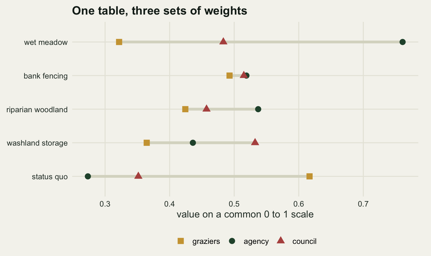
Four ways to add up three opinions
Four rules, all of them used in practice in one form or another, and none of them obviously wrong on inspection.
The first averages the weights and evaluates once: take the mean of the three weight vectors and score every alternative against it. The second evaluates three times and averages the values: give every party its own score column, then take the row means. The third is a Borda count, which throws away the numbers and keeps only each party’s ranking, awarding four points for a first place down to zero for a last. The fourth is minimax regret across parties: for each alternative, work out how far each party falls short of its own best option, take the worst of those three shortfalls, and pick the alternative whose worst shortfall is smallest.
score_pooled_w <- as.vector(V %*% colMeans(W))
score_mean_v <- rowMeans(sv)
place <- (n_alt + 1) - apply(sv, 2, rank)
borda <- rowSums(apply(sv, 2, rank) - 1)
regret <- sweep(-sv, 2, -apply(sv, 2, max), "-")
max_regret <- apply(regret, 1, max)

rules <- data.frame(pooled_weights = score_pooled_w, pooled_values = score_mean_v,
                    borda = borda, max_regret = max_regret, row.names = alt_name)
win <- c(pooled_weights = alt_name[which.max(score_pooled_w)],
         pooled_values = alt_name[which.max(score_mean_v)],
         borda = alt_name[which.max(borda)],
         minimax_regret = alt_name[which.min(max_regret)])

print(round(rules, 4))
pooled_weights pooled_values borda max_regret
status quo 0.4139 0.4139 4 0.4875
bank fencing 0.5089 0.5089 8 0.2420
wet meadow 0.5219 0.5219 6 0.2950
washland storage 0.4443 0.4443 6 0.3249
riparian woodland 0.4729 0.4729 6 0.2237print(place) graziers agency council
status quo 1 5 5
bank fencing 2 3 2
wet meadow 5 1 3
washland storage 4 4 1
riparian woodland 3 2 4print(round(regret, 4)) graziers agency council
status quo 0.0000 0.4875 0.1808
bank fencing 0.1239 0.2420 0.0174
wet meadow 0.2950 0.0000 0.0491
washland storage 0.2522 0.3249 0.0000
riparian woodland 0.1924 0.2237 0.0752print(win) pooled_weights pooled_values borda minimax_regret
"wet meadow" "wet meadow" "bank fencing" "riparian woodland" print(c(distinct_winners = length(unique(win))))distinct_winners
3 print(round(c(pooled_top_two_gap = -diff(sort(score_pooled_w, decreasing = TRUE)[1:2]),
borda_top_two_gap = -diff(sort(borda, decreasing = TRUE)[1:2]),
regret_top_two_gap = diff(sort(max_regret)[1:2])), 4)) pooled_top_two_gap borda_top_two_gap.wet meadow
0.0130 2.0000
regret_top_two_gap.bank fencing
0.0182 Three different recommendations come out of one table. Averaging the weights picks wet meadow, averaging the values picks wet meadow, the Borda count picks bank fencing, and minimax regret picks riparian woodland. Four rules, 3 distinct winners.
Say plainly how that example was built. I chose the numbers so that the rules would split, because a table where they happen to agree teaches nothing about what the rules do. The question worth answering is not whether such a table exists, which is now settled, but how common it is, and that comes later from a simulation over configurations I did not choose.
The mechanism is visible in the printed columns. Wet meadow wins the weighted average on 0.5219 against 0.5089 for bank fencing, a margin of 0.013, and it wins because the agency’s enthusiasm is large enough to carry the two parties who place it 5th and 3rd.
The Borda count cannot see enthusiasm. It sees that bank fencing is placed 2nd, 3rd and 2nd while wet meadow is placed 5th, 1st and 3rd, and it awards 8 points against 6. Minimax regret sees something else again: wet meadow leaves the graziers 0.295 short of their own best option, and riparian woodland, which is nobody’s favourite, leaves the worst-off party only 0.2237 short. Three rules, three different things being maximised, all of them defensible in a meeting.
The riparian woodland result is worth pausing on. It is best at nothing, it wins under neither averaging rule, and it takes only 6 Borda points. It wins minimax regret precisely because it is mediocre everywhere, and that is the rule doing what it was designed to do rather than a defect in the example.
Two averaging orders that turn out to be one
Practitioners argue about the first two rules. Should the group agree a set of weights and then run the model once, or should each member run the model and the group average the answers? The literature on group decision analysis treats these as distinct procedures with different behavioural properties, which they are. As arithmetic on this table they are the same operation.
The value of alternative \(a\) to party \(k\) is \(v_k(a) = \sum_j w_{kj} x_j(a)\) where \(x_j\) is the normalised score on objective \(j\). Averaging over \(K\) parties gives
\[\frac{1}{K}\sum_k v_k(a) = \frac{1}{K}\sum_k \sum_j w_{kj}\, x_j(a) = \sum_j \Big(\frac{1}{K}\sum_k w_{kj}\Big) x_j(a)\]
and the right-hand side is the score under the averaged weights. The sums commute, so the two rules are identical whenever the value function is linear in the normalised scores and every party uses the same normalisation.
lin_pooled <- as.vector(V %*% colMeans(W))
lin_individual <- rowMeans(V %*% t(W))
print(c(max_abs_difference = max(abs(lin_pooled - lin_individual))))
max_abs_difference
1.665335e-16 v_exp <- function(z, rho) {
if (abs(rho) < 1e-9) z else (1 - exp(-rho * z)) / (1 - exp(-rho))
}
rho <- c(graziers = -1.4, agency = 1.8, council = 0.52)
sv_curve <- sapply(stake, function(k) as.vector(v_exp(V, rho[k]) %*% W[k, ]))
rownames(sv_curve) <- alt_name
pool_first <- as.vector(v_exp(V, mean(rho)) %*% colMeans(W))
ind_first <- rowMeans(sv_curve)
ord <- data.frame(pooled_first = pool_first, individual_first = ind_first,
difference = pool_first - ind_first, row.names = alt_name)
print(round(rho, 3))graziers agency council
-1.40 1.80 0.52 print(round(sv_curve, 4)) graziers agency council
status quo 0.5499 0.4085 0.3857
bank fencing 0.3364 0.7040 0.5707
wet meadow 0.2344 0.8380 0.5308
washland storage 0.2468 0.6311 0.5860
riparian woodland 0.2764 0.7166 0.5166print(round(ord, 4)) pooled_first individual_first difference
status quo 0.4325 0.4480 -0.0155
bank fencing 0.5429 0.5370 0.0059
wet meadow 0.5434 0.5344 0.0090
washland storage 0.4758 0.4879 -0.0122
riparian woodland 0.5071 0.5032 0.0039print(c(pooled_winner = alt_name[which.max(pool_first)],
individual_winner = alt_name[which.max(ind_first)])) pooled_winner individual_winner
"wet meadow" "bank fencing" print(round(c(largest_score_difference = max(abs(ord$difference)),
pooled_top_two_gap =
-diff(sort(pool_first, decreasing = TRUE)[1:2])), 5))largest_score_difference pooled_top_two_gap
0.01549 0.00045 Under the linear model the largest difference between the two orders across all five alternatives is 1.67e-16, which is floating-point noise. They are not two rules. They are one rule computed two ways, and a workshop that spends an afternoon choosing between them has spent an afternoon on nothing.
They come apart as soon as the parties differ in more than their weights. Give each party an exponential value function on the normalised scores, \(v(z) = (1 - e^{-\rho z})/(1 - e^{-\rho})\), with its own curvature \(\rho\). The graziers get -1.4, a convex curve, which says a gross margin below viability is nearly worthless and only the top of the range counts. The agency gets 1.8, strongly concave, the diminishing returns of a conservation body that mostly wants a threshold cleared. The council gets 0.52, mildly concave. Pooling first now requires a single curve, and the only defensible one is the average curvature, 0.3067.
The two orders now give wet meadow and bank fencing respectively. Be honest about how thin that is. The largest score difference between the two orders is 0.01549, and the reason it flips the winner is that under the pooled-first calculation the top two alternatives are separated by 0.00045. The difference between the procedures is small; it decides the outcome because the decision was almost a tie.
How much curvature disagreement does it take? Sweep the three curvatures apart from a common value along a fixed direction and find where the two orders first part company.
rho_dir <- c(graziers = -1, agency = 1, council = 0.2)
spread <- seq(0, 2.4, by = 0.02)
sweep_out <- t(vapply(spread, function(s) {
  rr <- 0.2 + s * rho_dir
  sm <- sapply(stake, function(k) as.vector(v_exp(V, rr[k]) %*% W[k, ]))
  a2 <- as.vector(v_exp(V, mean(rr)) %*% colMeans(W))
  b2 <- rowMeans(sm)
  c(spread = s, max_diff = max(abs(a2 - b2)),
    agree = as.numeric(which.max(a2) == which.max(b2)))
}, numeric(3)))

first_flip <- sweep_out[which(sweep_out[, "agree"] == 0)[1], ]
print(round(head(sweep_out, 4), 6))
spread max_diff agree
[1,] 0.00 0.000000 1
[2,] 0.02 0.000167 1
[3,] 0.04 0.000334 1
[4,] 0.06 0.000503 1print(round(first_flip, 4)) spread max_diff agree
0.9000 0.0083 0.0000 print(round(c(diff_at_spread_one =
sweep_out[which.min(abs(spread - 1)), "max_diff"],
diff_at_largest_spread = sweep_out[nrow(sweep_out), "max_diff"]), 5)) diff_at_spread_one.max_diff diff_at_largest_spread.max_diff
0.00929 0.02389 At zero spread the difference is exactly zero, as the algebra requires. The winners first disagree at a spread of 0.9, where the largest score difference is still only 0.0083. At the far end of the sweep the difference has grown to 0.02389, still under two and a half per cent of the value scale. The two averaging orders are a small effect throughout, and the practical reading is that if they disagree on your table, the table has a near-tie in it and that is the finding worth reporting.
How often the rule picks the winner
One constructed example proves that rules can disagree. It says nothing about how often. The measurement that answers that keeps the consequence table fixed, because the ecology is not in dispute, and draws the three parties at random: three independent weight vectors uniform on the five-objective simplex, six thousand times over.
This is a different measurement from the one in the earlier posts in this cluster, and the difference is the whole point of this one. There the weight simplex belonged to a single decision maker and the question was how much of the recommendation survived that one person’s uncertainty about their own trade-offs. Here every draw is a complete, internally consistent, fully confident set of three decision makers who disagree with each other. The uncertainty being swept is not epistemic. It is the composition of the room.
set.seed(20260730)
n_trio <- 6000
draw_simplex <- function(n) {
  m <- matrix(rexp(n * n_obj), n, n_obj)
  m / rowSums(m)
}

Wk <- lapply(1:3, function(i) draw_simplex(n_trio))
Sk <- lapply(Wk, function(w) V %*% t(w))
S_mean <- (Sk[[1]] + Sk[[2]] + Sk[[3]]) / 3
S_pool <- V %*% t((Wk[[1]] + Wk[[2]] + Wk[[3]]) / 3)
B_sim <- Reduce(`+`, lapply(Sk, function(S) apply(S, 2, rank)))
R_sim <- Reduce(pmax, lapply(Sk, function(S) sweep(-S, 2, -apply(S, 2, max), "-")))

winner <- cbind(pooled_weights = max.col(t(S_pool), "first"),
                pooled_values = max.col(t(S_mean), "first"),
                borda = max.col(t(B_sim), "first"),
                minimax_regret = max.col(t(-R_sim), "first"))

print(c(trios = n_trio, pooled_vs_individual_gap = max(abs(S_pool - S_mean))))
trios pooled_vs_individual_gap
6.000000e+03 3.330669e-16 print(round(apply(winner, 2, function(v)
table(factor(v, 1:n_alt, alt_name)) / n_trio), 4)) pooled_weights pooled_values borda minimax_regret
status quo 0.0603 0.0603 0.0562 0.0413
bank fencing 0.1893 0.1893 0.3547 0.2843
wet meadow 0.6873 0.6873 0.5307 0.5853
washland storage 0.0613 0.0613 0.0527 0.0508
riparian woodland 0.0017 0.0017 0.0058 0.0382pr <- combn(4, 2)
disagree <- apply(pr, 2, function(ij) mean(winner[, ij[1]] != winner[, ij[2]]))
names(disagree) <- apply(pr, 2, function(ij)
paste(colnames(winner)[ij], collapse = " / "))
print(round(disagree, 4)) pooled_weights / pooled_values pooled_weights / borda
0.0000 0.2598
pooled_weights / minimax_regret pooled_values / borda
0.2027 0.2598
pooled_values / minimax_regret borda / minimax_regret
0.2027 0.3203 print(round(c(all_four_agree =
mean(apply(winner, 1, function(r) length(unique(r)) == 1)),
three_or_more_winners =
mean(apply(winner, 1, function(r) length(unique(r)) >= 3))), 4)) all_four_agree three_or_more_winners
0.6198 0.0225 The four rules name the same alternative in 61.98 per cent of the six thousand trios, so in most rooms the arithmetic does not matter. In the remaining 38.02 per cent it does, and in 2.25 per cent of all trios the four rules produce three or more distinct recommendations.
The pairwise rates are the table to keep. The Borda count disagrees with the weighted average in 25.98 per cent of trios and with minimax regret in 32.03 per cent, which is the worst pair in the matrix. Minimax regret disagrees with the weighted average in 20.27 per cent. And the two averaging orders, the pair that generates the most discussion, disagree in 0 per cent, because the largest gap between their scores over all six thousand trios and all five alternatives is 3.33e-16.
rule_lab <- c("average the\nweights", "average the\nvalues", "Borda\ncount",
              "minimax\nregret")
dm <- expand.grid(a = 1:4, b = 1:4)
dm$rate <- mapply(function(i, j)
  if (i == j) NA_real_ else mean(winner[, i] != winner[, j]), dm$a, dm$b)
dm$lab <- ifelse(is.na(dm$rate), "", sprintf("%.1f%%", 100 * dm$rate))
dm$a <- factor(rule_lab[dm$a], levels = rule_lab)
dm$b <- factor(rule_lab[dm$b], levels = rev(rule_lab))

ggplot(dm, aes(a, b, fill = rate)) +
  geom_tile(colour = "#f5f4ee", linewidth = 1.4) +
  geom_text(aes(label = lab, colour = !is.na(rate) & rate > 0.18),
            size = 4.1, show.legend = FALSE) +
  scale_fill_gradient(low = "#f0efe6", high = te_pal$forest, na.value = "#f5f4ee",
                      breaks = c(0, 0.1, 0.2, 0.3),
                      labels = c("0%", "10%", "20%", "30%"), name = "disagree") +
  scale_colour_manual(values = c("#2c3a31", "#f5f4ee")) +
  labs(x = NULL, y = NULL,
       title = "How often two rules name a different winner") +
  theme_te() +
  theme(panel.grid.major = element_blank(), plot.margin = margin(8, 12, 4, 8))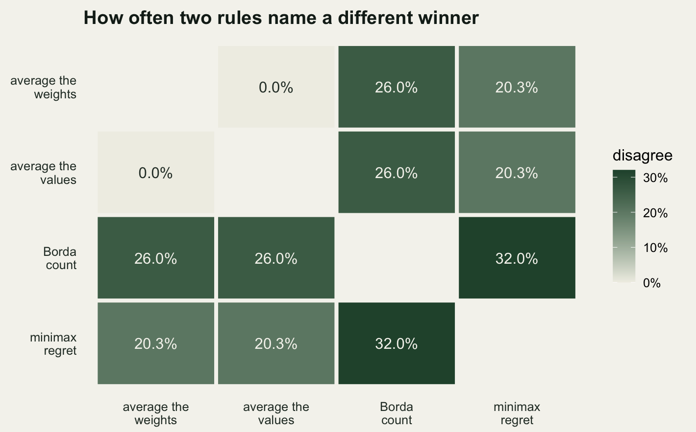
The winner shares in the printed table say something the disagreement rates do not. Wet meadow takes 68.73 per cent of trios under the weighted average but only 53.07 per cent under Borda, and bank fencing goes the other way, 18.93 per cent against 35.47 per cent. Rules are not noisy versions of each other. Each one has a systematic taste, and Borda’s taste is for the alternative that is nobody’s favourite and nobody’s last, which is a value judgement dressed as a counting procedure.
Where the majority goes round in a circle
The rules so far all return an answer. The pairwise majority does not always have one to return. Ask the three parties to compare two alternatives at a time and give the win to whichever gets two votes out of three. A Condorcet winner is an alternative that beats every other one in such a contest, and there are configurations where none exists, because the tournament contains a cycle.
beats <- array(FALSE, c(n_alt, n_alt, n_trio))
for (i in 1:n_alt) {
  for (j in 1:n_alt) {
    if (i != j) {
      beats[i, j, ] <- (Sk[[1]][i, ] > Sk[[1]][j, ]) +
        (Sk[[2]][i, ] > Sk[[2]][j, ]) + (Sk[[3]][i, ] > Sk[[3]][j, ]) >= 2
    }
  }
}
n_beaten <- apply(beats, c(1, 3), sum)
has_cw <- apply(n_beaten, 2, function(v) any(v == n_alt - 1))

tri <- combn(n_alt, 3)
in_cycle <- rep(FALSE, n_trio)
for (t in seq_len(ncol(tri))) {
  i <- tri[1, t]; j <- tri[2, t]; k <- tri[3, t]
  in_cycle <- in_cycle | (beats[i, j, ] & beats[j, k, ] & beats[k, i, ]) |
    (beats[i, k, ] & beats[k, j, ] & beats[j, i, ])
}
print(round(c(no_condorcet_winner = mean(!has_cw), some_three_cycle = mean(in_cycle),
              cycle_but_winner_exists = mean(in_cycle & has_cw)), 4))
no_condorcet_winner some_three_cycle cycle_but_winner_exists
0.0443 0.1192 0.0748 Out of 6000 trios, 4.43 per cent have no Condorcet winner at all. A three-cycle turns up somewhere in the tournament in 11.92 per cent, and in 7.48 per cent of trios a cycle exists lower down while an alternative at the top still beats everything. The second number is the one people quote; the first is the one that stops a decision.
The first trio in the simulation happens to be one of the failures, so no search was needed.
ic <- which(!has_cw)[1]
W_cyc <- do.call(rbind, lapply(Wk, function(w) w[ic, ]))
dimnames(W_cyc) <- list(c("party 1", "party 2", "party 3"), obj_name)
S_cyc <- V %*% t(W_cyc)

pair_tab <- outer(1:n_alt, 1:n_alt, Vectorize(function(i, j)
  if (i == j) NA_integer_ else sum(S_cyc[i, ] > S_cyc[j, ])))
dimnames(pair_tab) <- list(alt_name, alt_name)

print(c(trio_index = ic))
trio_index
1 print(round(W_cyc, 3)) waders phosphorus flood income access
party 1 0.011 0.387 0.396 0.023 0.183
party 2 0.184 0.155 0.073 0.359 0.228
party 3 0.056 0.241 0.463 0.153 0.087print(round(S_cyc, 4)) party 1 party 2 party 3
status quo 0.2260 0.5514 0.2808
bank fencing 0.5539 0.5390 0.4807
wet meadow 0.5700 0.5161 0.4643
washland storage 0.5162 0.3745 0.5270
riparian woodland 0.5542 0.4519 0.4920print(apply(S_cyc, 2, function(v) alt_name[order(-v)])) party 1 party 2 party 3
[1,] "wet meadow" "status quo" "washland storage"
[2,] "riparian woodland" "bank fencing" "riparian woodland"
[3,] "bank fencing" "wet meadow" "bank fencing"
[4,] "washland storage" "riparian woodland" "wet meadow"
[5,] "status quo" "washland storage" "status quo" print(pair_tab) status quo bank fencing wet meadow washland storage
status quo NA 1 1 1
bank fencing 2 NA 2 2
wet meadow 2 1 NA 2
washland storage 2 1 1 NA
riparian woodland 2 2 1 2
riparian woodland
status quo 1
bank fencing 1
wet meadow 2
washland storage 1
riparian woodland NAprint(c(beats_everything = sum(rowSums(pair_tab >= 2, na.rm = TRUE) == n_alt - 1)))beats_everything
0 Read the pairwise table along the top three contenders. Bank fencing beats wet meadow 2 votes to 1. Wet meadow beats riparian woodland 2 to 1. Riparian woodland beats bank fencing 2 to 1. Every one of those is a clear majority and together they close a loop, so the number of alternatives that beat all the others is 0.
None of the three parties is being awkward. Look at the printed orderings: each is a perfectly ordinary ranking produced by a perfectly ordinary weighted sum. The cycle is a property of the three of them together, and it means that on this configuration the phrase “what the majority prefers” does not refer to anything. Whichever alternative gets adopted, a majority would have preferred a different one. Choosing an aggregation rule at that point is not fine-tuning a recommendation; it is supplying the answer that the preferences do not contain.
How does the cycle rate depend on the length of the list? Extending the pool to eight alternatives, three of them combinations of the single actions, and sampling subsets lets us sweep it.
ext <- rbind(perf,
             "fencing and woodland" = c(32, 58, 28, 128, 22),
             "meadow and washland"  = c(56, 50, 40, 104, 20),
             "fencing and washland" = c(30, 46, 42, 122, 24))
Ve <- sweep(sweep(ext, 2, obj_lo, "-"), 2, obj_hi - obj_lo, "/")
print(round(Ve, 3))
waders phosphorus flood income access
status quo 0.233 0.133 0.08 0.929 0.65
bank fencing 0.367 0.733 0.32 0.486 0.70
wet meadow 0.967 0.867 0.28 0.129 0.60
washland storage 0.517 0.317 0.76 0.200 0.45
riparian woodland 0.400 0.800 0.40 0.371 0.40
fencing and woodland 0.533 0.967 0.56 0.200 0.55
meadow and washland 0.933 0.833 0.80 0.029 0.50
fencing and washland 0.500 0.767 0.84 0.157 0.60print(c(pool_size = nrow(Ve), dominated = sum(dominated(Ve))))pool_size dominated
8 0 set.seed(20260731)
n_rep <- 4000
no_cw_rate <- function(m) {
cnt <- 0L
for (r in seq_len(n_rep)) {
Vm <- Ve[sample.int(nrow(Ve), m), , drop = FALSE]
ww <- matrix(rexp(3 * n_obj), 3, n_obj)
S <- Vm %*% t(ww / rowSums(ww))
bt <- matrix(FALSE, m, m)
for (i in 1:m) for (j in 1:m) if (i != j) bt[i, j] <- sum(S[i, ] > S[j, ]) >= 2
if (!any(rowSums(bt) == m - 1)) cnt <- cnt + 1L
}
cnt / n_rep
}
m_seq <- 3:8
cyc_tab <- data.frame(alternatives = m_seq,
no_condorcet_winner = vapply(m_seq, no_cw_rate, numeric(1)))
print(round(cyc_tab, 4)) alternatives no_condorcet_winner
1 3 0.0132
2 4 0.0310
3 5 0.0475
4 6 0.0735
5 7 0.0843
6 8 0.1140print(round(c(replicates_each = n_rep,
slope_per_alternative =
unname(coef(lm(no_condorcet_winner ~ alternatives, cyc_tab))[2])), 5)) replicates_each slope_per_alternative
4.00e+03 1.97e-02 ggplot(cyc_tab, aes(alternatives, no_condorcet_winner)) +
geom_hline(yintercept = mean(!has_cw), colour = te_pal$clay, linetype = "22") +
geom_line(colour = te_pal$forest, linewidth = 0.8) +
geom_point(colour = te_pal$forest, size = 2.6) +
annotate("text", x = 3.05, y = mean(!has_cw) + 0.007, hjust = 0, size = 3.4,
colour = te_pal$clay,
label = sprintf("the five real alternatives: %.1f%%",
100 * mean(!has_cw))) +
scale_y_continuous(breaks = c(0, 0.05, 0.10),
labels = c("0%", "5%", "10%"), limits = c(0, 0.13)) +
scale_x_continuous(breaks = 3:8) +
labs(x = "alternatives on the table", y = "trios with no majority winner",
title = "Cycles get more common as the list grows") +
theme_te() +
theme(plot.margin = margin(8, 16, 4, 8))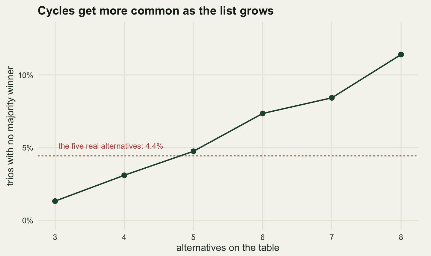
The rate climbs from 1.32 per cent at three alternatives to 11.4 per cent at eight, close enough to a straight line that a fitted slope of 1.97 percentage points per alternative summarises it. Generating more options is standard advice in structured decision making and it is good advice, because a wider set contains better alternatives. The measurement says it also makes a majority failure more likely, and both things are true at once.
What this reversal is not
Two earlier posts in this cluster measured something that also gets called rank reversal, and the mechanism there was different. In Structured decision making in R the scores were normalised against the best and worst values present in the alternative set, so adding a dominated option that set a new extreme on some objective moved a scale endpoint and reshuffled everything else. That is a single decision maker, a single set of weights, and an arithmetic artefact of data-dependent scaling. Every score in this post is computed against fixed natural bounds decided before the alternatives were listed, so that mechanism is switched off here by construction. The reversals measured above are caused by pooling several decision makers, and the two effects are independent: a group analysis with min-max scaling gets both, and neither one implies the other.
The distinction is testable. Drop one alternative that no rule recommends, keep the fixed bounds so no score changes, and see which rules move.
set.seed(20260801)
changed <- matrix(NA, n_trio, 3)
colnames(changed) <- c("pooled_values", "borda", "minimax_regret")
was_favourite <- rep(NA, n_trio)
fav <- do.call(rbind, lapply(Sk, function(S) max.col(t(S), "first")))

for (t in seq_len(n_trio)) {
  cand <- setdiff(1:n_alt, unique(winner[t, ]))
  if (!length(cand)) next
  drop_i <- cand[sample.int(length(cand), 1)]
  was_favourite[t] <- drop_i %in% fav[, t]
  keep <- setdiff(1:n_alt, drop_i)
  S2 <- cbind(Sk[[1]][keep, t], Sk[[2]][keep, t], Sk[[3]][keep, t])
  w_v <- keep[which.max(rowMeans(S2))]
  w_b <- keep[which.max(rowSums(apply(S2, 2, rank)))]
  w_r <- keep[which.min(apply(sweep(-S2, 2, -apply(S2, 2, max), "-"), 1, max))]
  changed[t, ] <- c(w_v, w_b, w_r) != winner[t, c(2, 3, 4)]
}

usable <- !is.na(changed[, 1])
print(c(usable_trios = sum(usable)))
usable_trios
6000 print(round(c(share_dropped_was_a_favourite = mean(was_favourite[usable])), 4))share_dropped_was_a_favourite
0.2705 print(round(colMeans(changed[usable, ]), 4)) pooled_values borda minimax_regret
0.0000 0.0627 0.0498 print(round(c(regret_if_favourite =
mean(changed[usable & was_favourite, "minimax_regret"]),
regret_if_not = mean(changed[usable & !was_favourite, "minimax_regret"]),
borda_if_favourite = mean(changed[usable & was_favourite, "borda"]),
borda_if_not = mean(changed[usable & !was_favourite, "borda"])), 4))regret_if_favourite regret_if_not borda_if_favourite borda_if_not
0.1842 0.0000 0.0240 0.0770 The weighted average never moves: 0 per cent, exactly, because with fixed bounds an alternative’s score does not depend on what else is on the list. The Borda count changes its recommendation in 6.27 per cent of trios and minimax regret in 4.98 per cent, and neither of those involves a single altered number in the consequence table.
The two mechanisms are cleanly separated in the conditional rates. Minimax regret changes in 18.42 per cent of the cases where the discarded option was some party’s own top choice, and in exactly 0 per cent otherwise, which is what the formula predicts: the rule reads the set only through each party’s best, so removing anything else is invisible to it. Borda goes the other way. It changes in 2.4 per cent of the cases where the dropped option was a favourite and 7.7 per cent where it was not, because what moves a Borda count is an option sitting between two others in different places for different parties, and a middling option does that more often than a leader does.
This is the independence of irrelevant alternatives condition failing, in the group setting, with the scaling artefact removed. Arrow’s theorem says that a rule which never does this, while also respecting unanimity and refusing to let one party decide everything, does not exist for three or more alternatives. The two rules above pay the bill in different currencies. The weighted average keeps independence and pays by requiring that one party’s value units be added to another’s, an exchange rate no measurement supplies. Borda refuses the exchange rate and pays in set dependence.
The price of a choice that does not depend on the rule
There is an escape that gets recommended in practice: stop looking for the best option and take the one that leaves the worst-off party least badly off. That choice can be defended without an aggregation rule, so it sidesteps everything above. The question this post is for is what it costs, and the answer is measurable on the same six thousand trios.
For every trio, work out the highest mean value available and how far each alternative falls short of it. That is the price. Then, for every alternative, take the regret of the worst-off party across all trios. That is what the price buys.
best_mean <- apply(S_mean, 2, max)
shortfall <- sweep(-S_mean, 2, -best_mean, "-")
front <- data.frame(
  alternative = alt_name,
  mean_value = rowMeans(S_mean),
  pct_shortfall = 100 * rowMeans(shortfall / rep(best_mean, each = n_alt)),
  worst_regret = apply(R_sim, 1, max),
  regret_q95 = apply(R_sim, 1, quantile, 0.95),
  win_share = as.vector(table(factor(winner[, 1], 1:n_alt)) / n_trio))

i_rob <- which.min(front$worst_regret)
i_util <- which.max(front$mean_value)
i_q95 <- which.min(front$regret_q95)

print(round(front[, -1], 4))
mean_value pct_shortfall worst_regret regret_q95 win_share
status quo 0.4046 29.6914 0.7070 0.5903 0.0603
bank fencing 0.5216 10.1927 0.5439 0.3611 0.1893
wet meadow 0.5682 3.0208 0.7300 0.3904 0.6873
washland storage 0.4487 22.4530 0.6707 0.4386 0.0613
riparian woodland 0.4748 18.3272 0.5245 0.3790 0.0017print(c(minimax_regret_choice = alt_name[i_rob],
highest_average_choice = alt_name[i_util],
percentile_choice = alt_name[i_q95])) minimax_regret_choice highest_average_choice percentile_choice
"riparian woodland" "wet meadow" "bank fencing" print(round(c(value_given_up = front$pct_shortfall[i_rob] - front$pct_shortfall[i_util],
regret_bought = front$worst_regret[i_util] - front$worst_regret[i_rob]), 4))value_given_up regret_bought
15.3064 0.2055 print(round(c(second_best_excess_regret =
front$worst_regret[2] - front$worst_regret[i_rob],
second_best_value_recovered =
front$pct_shortfall[i_rob] - front$pct_shortfall[2]), 4)) second_best_excess_regret second_best_value_recovered
0.0193 8.1345 The strict answer is riparian woodland, the alternative that is best at nothing. Committing to it in advance costs 18.33 per cent of the mean value available, averaged over trios, against 3.02 per cent for wet meadow, which has the highest average value. That is 15.31 percentage points of value handed over. What it buys is a fall in the worst-off party’s regret from 0.73 to 0.5245, a reduction of 0.2055 on the same zero to one scale. Whether that is a good trade is a judgement, but at least it is a judgement about two numbers rather than about a rule.
The deal on offer is worse than the strict rule makes it look. Bank fencing has a worst-case regret of 0.5439, only 0.0193 above the minimum, and it gives back 8.13 of those 15.31 percentage points. Buying the last sliver of worst-case protection is where just over half the money goes, which is the usual shape of a minimax criterion and a good reason to plot the frontier rather than run the rule.
fr <- data.frame(x = rep(front$pct_shortfall, 2),
                 y = c(front$worst_regret, front$regret_q95),
                 criterion = rep(c("worst case over all trios",
                                   "95th percentile of the trios"), each = n_alt))

ggplot(fr, aes(x, y)) +
  geom_segment(data = front, inherit.aes = FALSE,
               aes(x = pct_shortfall, xend = pct_shortfall,
                   y = regret_q95, yend = worst_regret),
               colour = te_pal$line, linewidth = 1.2) +
  geom_point(aes(colour = criterion, shape = criterion), size = 3.2) +
  geom_text(data = front, inherit.aes = FALSE,
            aes(pct_shortfall, worst_regret, label = alternative),
            vjust = -1.1, size = 3.3, colour = "#2c3a31") +
  scale_colour_manual(values = c(te_pal$gold, te_pal$clay), name = NULL) +
  scale_shape_manual(values = c(17, 16), name = NULL) +
  scale_y_continuous(limits = c(0.3, 0.82)) +
  scale_x_continuous(limits = c(-1, 34)) +
  labs(x = "average shortfall from the best available mean value (per cent)",
       y = "regret of the worst-off party",
       title = "What robustness costs, and how it is defined") +
  theme_te() +
  theme(legend.position = "bottom", plot.margin = margin(8, 18, 4, 8))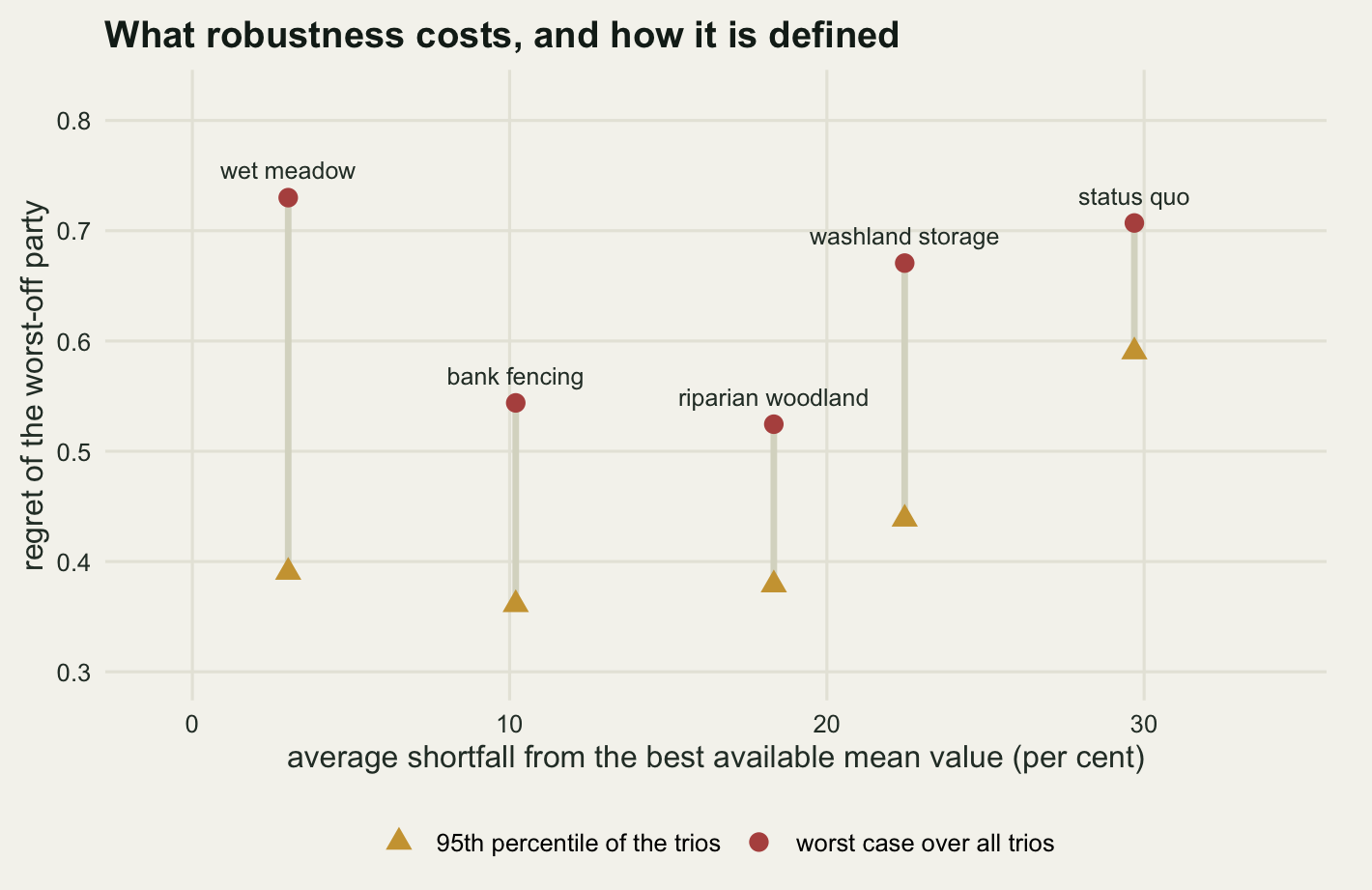
Then the escape route closes. Define the worst case as the ninety fifth percentile of the trios rather than the maximum, which is the more defensible statistic when the extreme trios are configurations of parties nobody expects to meet, and the recommendation moves from riparian woodland to bank fencing, whose percentile regret is 0.3611 against 0.379. The robust choice is itself a function of how robustness is defined, and that is the same problem one level up. There is no rule-free place to stand; there is only a choice made in the open instead of by default.
That is worth stating without softening it, because the practical advice in the literature, which I set out to confirm, does not survive the measurement intact. Choosing for robustness does not remove the arbitrary step. It replaces the choice of an aggregation rule with the choice of a worst-case statistic, and on this table the two choices move the recommendation by a comparable amount.
What to take away
Three parties, one agreed consequence table, and four sensible ways of adding up their preferences give 3 different recommendations. Over six thousand random configurations of three parties the four rules all agree 61.98 per cent of the time, which is reassuring, and the pairs that disagree do so systematically rather than occasionally: 32.03 per cent for the worst pair. In 4.43 per cent of configurations there is no majority winner at all, and that rate rises by about 1.97 percentage points for every alternative added to the list.
Two results went against what I expected before running them. The argument practitioners actually have, whether to average the weights or average the individual scores, is not an argument: the two orders differ by 3.33e-16 across the whole simulation and pick different winners in 0 per cent of trios, and they only come apart when the parties differ in the curvature of their value functions, and even then only where the table has a near-tie at the top: in the worked example the top two alternatives sat 0.00045 apart. And the standard escape hatch leaks: the alternative that minimises the maximum regret costs 15.31 percentage points of average value, and switching from the maximum to the ninety fifth percentile changes which alternative that is.
What survives is a short procedure. Fix the normalisation bounds before listing the alternatives, so that nothing you measure afterwards is scaling. Compute the winner under at least two aggregation rules with different characters, one that uses magnitudes and one that uses only ranks. If they agree, say so and move on, which will happen most of the time. If they disagree, do not pick the rule that gives the answer you prefer; report both, add the pairwise majority table, and put the disagreement itself in front of the group, because a group that can see the shape of its own disagreement is in a better position than one handed a single number.
The limits of all this are worth setting out, because they are not small. Every party here is represented by a linear additive value model over the same five objectives, elicited without error, and real weight elicitation is worse than that by a wide margin: the gap between the top two alternatives under the pooled weights was 0.013 on a zero to one scale, comfortably inside the error of any elicitation protocol I know of, which means the rule choice and the elicitation error are contending for the same margin. The simulation draws the three parties independently and uniformly, which is the most disagreeable room possible; real stakeholders share a culture and correlate, so the rates above are an upper bound rather than a forecast. Three of the four rules require adding one party’s value units to another’s, and nothing in the ecology, the hydrology or the farm accounts supplies that exchange rate. And no simulation can prove an impossibility theorem. Arrow’s result is a proof about rules, and what the numbers here can do is show you what the proof costs on one small catchment problem where every fact is agreed.
References
Arrow KJ 1950 Journal of Political Economy 58(4):328-346 (10.1086/256963)
Arrow KJ 1963 Social Choice and Individual Values, second edition. Yale University Press, ISBN 978-0-300-01364-1
Dyer JS, Sarin RK 1979 Management Science 25(9):822-832 (10.1287/mnsc.25.9.822)
Keeney RL 2013 Decision Analysis 10(2):103-120 (10.1287/deca.2013.0265)
Keeney RL, Raiffa H 1993 Decisions with Multiple Objectives: Preferences and Value Tradeoffs. Cambridge University Press, ISBN 978-0-521-44185-8
Gregory R, Failing L, Harstone M, Long G, McDaniels T, Ohlson D 2012 Structured Decision Making: A Practical Guide to Environmental Management Choices. Wiley-Blackwell, ISBN 978-1-4443-3341-1
Davies AL, Bryce R, Redpath SM 2013 Conservation Biology 27(5):936-944 (10.1111/cobi.12090)
Redpath SM, Young J, Evely A, Adams WM, Sutherland WJ, Whitehouse A, Amar A, Lambert RA, Linnell JDC, Watt A, Gutierrez RJ 2013 Trends in Ecology and Evolution 28(2):100-109 (10.1016/j.tree.2012.08.021)
Regan HM, Ben-Haim Y, Langford B, Wilson WG, Lundberg P, Andelman SJ, Burgman MA 2005 Ecological Applications 15(4):1471-1477 (10.1890/03-5419)