library(ggplot2)
library(patchwork)

te_paper  <- "#f5f4ee"
te_ink    <- "#16241d"
te_body   <- "#2c3a31"
te_forest <- "#275139"
te_rust   <- "#b5534e"
te_gold   <- "#c9b458"
te_line   <- "#dad9ca"

theme_datasheet <- function() {
  theme_minimal(base_size = 12) +
    theme(plot.background  = element_rect(fill = te_paper, colour = NA),
          panel.background = element_rect(fill = te_paper, colour = NA),
          panel.grid.major = element_line(colour = te_line, linewidth = 0.3),
          panel.grid.minor = element_blank(),
          text             = element_text(colour = te_body),
          plot.title       = element_text(colour = te_ink, face = "bold"),
          plot.subtitle    = element_text(colour = te_body),
          axis.text        = element_text(colour = te_body))
}Transients and the single-capture rule in CJS
R
capture-recapture
survival analysis
population ecology
ecology tutorial
Deleting birds caught only once before a CJS fit makes survival a readout of detection and study length. The two-age model and TEST 3.SR instead, in R.
A reedbed ringing station runs its nets through the breeding season. Every year a large share of the reed warblers ringed there are never caught again: some die, some were missed, and a good many were passage birds on their way somewhere else, caught once in a net that happened to stand on their route. When the capture histories go into a Cormack-Jolly-Seber (CJS) model, those passing birds are a problem, because the model reads an animal that is never seen again as an animal that probably died. The shortcut that is easy to reach for is to delete every bird caught only once, on the reasoning that the transients are exactly the birds with a single capture, and to fit the CJS model to whatever is left.
The trouble with the shortcut is known, and so is the repair. Pradel, Hines, Lebreton and Nichols (1997) set out capture-recapture survival models that take account of transients: they give the first interval after marking its own survival parameter, which absorbs the passing birds, and leave the survival of the residents to a second parameter estimated from everything else. They also showed that one of the standard goodness-of-fit components, TEST 3.SR, is the one transients disturb, which makes it a diagnostic for them, and U-CARE (Choquet and colleagues 2009) computes it from a capture history file. This post is a demonstration of that work, built by hand in base R. What it measures is the part that a reader tempted by the deletion rule would want in numbers: how the estimate after deletion depends on the detection probability and on the number of occasions, whether it still follows the true survival at all, and what the discarded marks cost.
The site already has the neighbouring result. Joint live-dead models already showed that a live-only model returns survival times fidelity, and that a first-interval rate different from the adult one produces a blend belonging to no interval of the study. That post owns the damage emigration does to an undeleted CJS fit: it proves the constant-fidelity case as an identity, and shows with a simulated natal-dispersal case that a first-interval departure gives a blend no interval owns, which is the transient case here. This post is about the rule an analyst reaches for to avoid that blend, and about the fact that the rule answers a question about the survey rather than about the birds.
The other neighbour is Jolly-Seber and POPAN, which makes the point that CJS conditions on first capture and that this conditioning is legitimate: how an animal came to be marked never enters the likelihood, and nothing about survival depends on it. The deletion rule conditions on something else. It keeps an animal according to whether it was caught again, and whether it was caught again is the response the survival model is fitted to. The basic CJS model is the one Cormack-Jolly-Seber survival models in R fits from an m-array; the form used below, three numbers per animal and a chi term for never being seen again, is the one the Jolly-Seber post writes out, here tabulated as sufficient statistics so that thousands of simulated studies fit in a few seconds. The post on delayed entry and the Weibull hazard shape deals with animals that died before anyone could mark them, a selection made by nature before the study began; here the analyst makes it after the data are in.
A ringing study with passage birds
Each simulated study has K capture occasions and releases 120 newly ringed birds at every occasion except the last. A share tau of each release are transients: they leave for good immediately after being ringed and can never be caught again. The rest are residents, which survive each interval with probability phi and, while alive, are caught at each later occasion with probability p. Survival here is per-interval apparent survival, the quantity any live-only model estimates; it is not annual survival unless the occasions are a year apart, and it is not a study-wide proportion.
sim_study <- function(k_occ, n_rel, phi, p_det, tau) {
  first    <- rep(seq_len(k_occ - 1), each = n_rel)
  n_mark   <- length(first)
  alive    <- runif(n_mark) >= tau
  hist_mat <- matrix(0L, n_mark, k_occ)
  hist_mat[cbind(seq_len(n_mark), first)] <- 1L
  for (occ in 2:k_occ) {
    at_risk <- first < occ
    alive[at_risk] <- alive[at_risk] & (runif(sum(at_risk)) < phi)
    seen <- at_risk & alive & (runif(n_mark) < p_det)
    hist_mat[seen, occ] <- 1L
  }
  list(hist = hist_mat, first = first, k_occ = k_occ)
}
The notation and the model family are those of Lebreton, Burnham, Clobert and Anderson (1992). The CJS likelihood conditional on first release needs only three numbers per animal: the occasion of first release, the occasion of last capture and the number of recaptures in between. An animal last seen at occasion l contributes the probability chi[l] of never being seen again after it, and chi comes from a backward recursion: either the animal dies in the next interval, or it survives, is missed, and is never seen from the occasion after. Every death the model learns about is inside those chi terms.
The two-age-class model of Pradel and colleagues changes one thing. Survival over the first interval after marking is phi_one, and every later interval is phi_two. An animal never recaptured after its first release gets its own chi_one, which starts with phi_one and then hands over to the resident recursion. With transients leaving at marking, phi_one should come out at (1 - tau) * phi and phi_two at phi; that identity is the calibration for the fit, not a finding.
suff_stats <- function(hist_mat, first, k_occ) {
  last <- max.col(hist_mat, ties.method = "last")
  n_re <- rowSums(hist_mat) - 1L
  key  <- (first - 1L) * k_occ^2 + (last - 1L) * k_occ + n_re
  tab  <- tabulate(key + 1L, nbins = k_occ^3)
  idx  <- which(tab > 0) - 1L
  list(first = idx %/% k_occ^2 + 1L, last = (idx %/% k_occ) %% k_occ + 1L,
       n_re = idx %% k_occ, w = tab[tab > 0], k_occ = k_occ)
}

chi_rec <- function(phi, p_det, k_occ) {
  chi <- numeric(k_occ)
  chi[k_occ] <- 1
  for (occ in (k_occ - 1):1) chi[occ] <- (1 - phi) + phi * (1 - p_det) * chi[occ + 1]
  chi
}

nll_cjs <- function(par, st) {
  phi <- plogis(par[1]); p_det <- plogis(par[2])
  chi <- chi_rec(phi, p_det, st$k_occ)
  gap <- st$last - st$first
  -sum(st$w * (gap * log(phi) + st$n_re * log(p_det) +
               (gap - st$n_re) * log(1 - p_det) + log(chi[st$last])))
}

nll_tsm <- function(par, st) {
  phi_one <- plogis(par[1]); phi_two <- plogis(par[2]); p_det <- plogis(par[3])
  chi_two <- chi_rec(phi_two, p_det, st$k_occ)
  chi_one <- c((1 - phi_one) + phi_one * (1 - p_det) * chi_two[-1], 1)
  gap  <- st$last - st$first
  surv <- ifelse(gap == 0, 0, log(phi_one) + pmax(gap - 1, 0) * log(phi_two))
  chiv <- ifelse(gap == 0, chi_one[st$last], chi_two[st$last])
  -sum(st$w * (surv + st$n_re * log(p_det) +
               (gap - st$n_re) * log(1 - p_det) + log(chiv)))
}

wald_logit <- function(fit, j) {
  v_j <- tryCatch(diag(solve(fit$hessian))[j], error = function(e) NA_real_)
  if (!is.finite(v_j) || v_j <= 0) return(c(NA_real_, NA_real_))
  plogis(fit$par[j] + c(-1, 1) * qnorm(0.975) * sqrt(v_j))
}

fit_cjs <- function(st, ci = FALSE) {
  fit <- optim(c(1, 0), nll_cjs, st = st, method = "BFGS", hessian = ci)
  if (!ci) return(plogis(fit$par[1]))
  c(plogis(fit$par[1]), wald_logit(fit, 1))
}

fit_tsm <- function(st, ci = FALSE) {
  fit <- optim(c(0, 1, 0), nll_tsm, st = st, method = "BFGS", hessian = ci)
  if (!ci) return(plogis(fit$par[1:2]))
  c(plogis(fit$par[1:2]), wald_logit(fit, 2))
}
Every study is analysed four ways. The first is the constant CJS on the full histories. The second deletes every bird with exactly one capture and fits the same CJS to the rest: this is the rule. The third keeps the same birds as the rule but also removes each bird’s first capture, so that its history starts at its second capture. Leaving out each animal’s first capture is an ad hoc approach discussed by Pradel and colleagues (1997) alongside their two-age model; here it is used to locate the damage, and it comes back in a later section. The fourth is the two-age model on the full, undeleted histories.
analyse <- function(sim, ci = FALSE, gof = FALSE) {
  k_occ <- sim$k_occ
  keep  <- rowSums(sim$hist) >= 2
  st_full <- suff_stats(sim$hist, sim$first, k_occ)
  st_del  <- suff_stats(sim$hist[keep, , drop = FALSE], sim$first[keep], k_occ)
  h_sec <- sim$hist[keep, , drop = FALSE]
  h_sec[cbind(seq_len(nrow(h_sec)), sim$first[keep])] <- 0L
  st_sec <- suff_stats(h_sec, max.col(h_sec, ties.method = "first"), k_occ)
  out <- c(pct_del   = 100 * mean(!keep),
           pct_first = 100 * mean(!keep[sim$first == 1]),
           pct_last  = 100 * mean(!keep[sim$first == k_occ - 1]))
  if (!ci) {
    tsm <- fit_tsm(st_full)
    out <- c(out, full = fit_cjs(st_full), del = fit_cjs(st_del),
             sec = fit_cjs(st_sec), tsm_one = tsm[1], tsm_two = tsm[2])
  } else {
    f_full <- fit_cjs(st_full, TRUE); f_del <- fit_cjs(st_del, TRUE)
    f_sec  <- fit_cjs(st_sec, TRUE);  f_tsm <- fit_tsm(st_full, TRUE)
    out <- c(out, full = f_full[1], full_lo = f_full[2], full_hi = f_full[3],
             del = f_del[1], del_lo = f_del[2], del_hi = f_del[3],
             sec = f_sec[1], sec_lo = f_sec[2], sec_hi = f_sec[3],
             tsm_one = f_tsm[1], tsm_two = f_tsm[2],
             tsm_lo = f_tsm[3], tsm_hi = f_tsm[4])
  }
  if (gof) out <- c(out, test_3sr(sim$hist, sim$first, k_occ))
  out
}

run_cell <- function(n_rep, k_occ, phi, p_det, tau, ci = FALSE, gof = FALSE) {
  t(replicate(n_rep, analyse(sim_study(k_occ, n_rel, phi, p_det, tau), ci, gof)))
}
When gof = TRUE the study also gets the transient diagnostic TEST 3.SR, which is set out in the last analysis section; the function is defined here because the anchor runs below call it.
test_3sr <- function(hist_mat, first, k_occ) {
  seen_after <- t(apply(hist_mat[, k_occ:1, drop = FALSE], 1, cummax))[, k_occ:1]
  x_two <- z_part <- numeric(0)
  for (occ in 2:(k_occ - 1)) {
    caught <- hist_mat[, occ] == 1L
    again  <- seen_after[, occ + 1] == 1L
    is_new <- first == occ
    tab <- c(sum(caught & is_new & again), sum(caught & is_new & !again),
             sum(caught & !is_new & again), sum(caught & !is_new & !again))
    n_new <- tab[1] + tab[2]; n_old <- tab[3] + tab[4]
    n_ag  <- tab[1] + tab[3]; n_no  <- tab[2] + tab[4]
    if (min(n_new, n_old, n_ag, n_no) == 0) next
    stat <- (n_new + n_old) * (tab[1] * tab[4] - tab[2] * tab[3])^2 /
      (n_new * n_old * n_ag * n_no)
    x_two  <- c(x_two, stat)
    z_part <- c(z_part, sign(tab[3] / n_old - tab[1] / n_new) * sqrt(stat))
  }
  c(chi = sum(x_two), df = length(x_two), z = sum(z_part) / sqrt(length(z_part)))
}
One study at the anchor design shows the four readings side by side: six occasions, detection 0.45, resident survival 0.80, and a quarter of every release transient.
n_rel      <- 120
k_anchor   <- 6
p_anchor   <- 0.45
phi_anchor <- 0.80
tau_anchor <- 0.25

set.seed(6021)
worked_sim <- sim_study(k_anchor, n_rel, phi_anchor, p_anchor, tau_anchor)
worked     <- analyse(worked_sim)
n_marks    <- nrow(worked_sim$hist)
n_deleted  <- sum(rowSums(worked_sim$hist) == 1)
Of the 600 birds ringed in this study, 362 (60.3 per cent) were caught only once and are deleted by the rule. The full CJS gives an apparent survival of 0.709, below the resident value of 0.80 because the transients count as deaths: that is the blend the joint live-dead post describes. The CJS after deletion gives 0.964. The two-age model gives 0.806 for residents and 0.561 for the first interval after ringing, where the identity predicts 0.600. The history restarted at the second capture gives 0.833.
The deletion share has a denominator that needs stating, because it is not a property of the birds alone. It is taken over all marks released, and that includes the birds ringed at the last release occasion, which have exactly one chance of a recapture. In this study 75.8 per cent of that final cohort were singletons against 57.5 per cent of the birds ringed at the first occasion. A study that ringed only at its first occasion, or that ran two more seasons, would report a different deletion share for the same population.
The two-age model passes its calibration
Repeating the anchor study at each of three transient shares gives the first comparison. Resident survival stays at 0.80 throughout; only the share of passing birds changes.
n_anchor <- 200
tau_grid <- c(0, 0.25, 0.40)
set.seed(9707)
anchor_runs <- lapply(tau_grid, function(tau_i)
  run_cell(n_anchor, k_anchor, phi_anchor, p_anchor, tau_i, ci = TRUE, gof = TRUE))

cover <- function(a, lo, hi) mean(a[, lo] <= phi_anchor & a[, hi] >= phi_anchor, na.rm = TRUE)
width <- function(a, lo, hi) mean(a[, hi] - a[, lo], na.rm = TRUE)
anchor_tab <- do.call(rbind, lapply(seq_along(tau_grid), function(i) {
  a <- anchor_runs[[i]]
  data.frame(tau = tau_grid[i], full = mean(a[, "full"]), del = mean(a[, "del"]),
             sec = mean(a[, "sec"]), tsm_two = mean(a[, "tsm_two"]),
             tsm_one = mean(a[, "tsm_one"]), one_pred = (1 - tau_grid[i]) * phi_anchor,
             tsm_one_se = sd(a[, "tsm_one"]) / sqrt(n_anchor),
             pct_del = mean(a[, "pct_del"]), pct_first = mean(a[, "pct_first"]),
             pct_last = mean(a[, "pct_last"]),
             sd_full = sd(a[, "full"]), sd_del = sd(a[, "del"]),
             sd_sec = sd(a[, "sec"]), sd_tsm = sd(a[, "tsm_two"]),
             w_full = width(a, "full_lo", "full_hi"), w_del = width(a, "del_lo", "del_hi"),
             w_sec = width(a, "sec_lo", "sec_hi"), w_tsm = width(a, "tsm_lo", "tsm_hi"),
             cov_full = cover(a, "full_lo", "full_hi"), cov_del = cover(a, "del_lo", "del_hi"),
             cov_sec = cover(a, "sec_lo", "sec_hi"), cov_tsm = cover(a, "tsm_lo", "tsm_hi"),
             n_fail = sum(is.na(a[, c("full_lo", "del_lo", "sec_lo", "tsm_lo")])),
             rej_chi = mean(a[, "chi"] > qchisq(0.95, a[, "df"])),
             rej_z = mean(a[, "z"] > qnorm(0.95)))
}))
calib_gap <- max(abs(anchor_tab$tsm_one - anchor_tab$one_pred))
calib_z   <- max(abs(anchor_tab$tsm_one - anchor_tab$one_pred) / anchor_tab$tsm_one_se)
round(anchor_tab[, c("tau", "full", "del", "sec", "tsm_two", "tsm_one", "one_pred", "pct_del")], 3)
tau full del sec tsm_two tsm_one one_pred pct_del
1 0.00 0.801 0.961 0.803 0.801 0.802 0.80 45.653
2 0.25 0.726 0.960 0.798 0.800 0.600 0.60 59.377
3 0.40 0.677 0.961 0.803 0.804 0.478 0.48 67.485The calibration holds. Averaged over 200 studies, the two-age first-interval estimate reads 0.802, 0.600 and 0.478 at transient shares of 0.00, 0.25 and 0.40, against 0.800, 0.600 and 0.480 from (1 - tau) * phi; the largest gap is 0.002, or 1.0 Monte Carlo standard errors. The resident estimate reads 0.801, 0.800 and 0.804. The likelihood is doing what Pradel and colleagues say it does.
The full CJS falls from 0.801 to 0.677 as the transient share rises, which is the blend again. The deletion rule reads 0.961, 0.960 and 0.961. That flat line is the rule doing the job it was chosen for: the transients no longer pull the estimate down. It sits at the wrong level, though, and it sits there even at a transient share of zero, where there was nothing to remove and the full CJS was already right. The rule deleted 45.7 per cent of the marks in a study with no transients in it.
arm_lab <- c(full = "CJS, full histories", del = "CJS, singletons deleted",
             tsm_two = "two-age model, residents")
anchor_long <- do.call(rbind, lapply(names(arm_lab), function(nm)
  data.frame(tau = anchor_tab$tau, est = anchor_tab[[nm]], arm = arm_lab[[nm]])))
anchor_long$arm <- factor(anchor_long$arm, levels = arm_lab)

p_left <- ggplot(anchor_long, aes(tau, est, colour = arm)) +
  geom_hline(yintercept = phi_anchor, linetype = "dashed", colour = te_body, linewidth = 0.5) +
  geom_line(linewidth = 0.9) +
  geom_point(size = 2.6) +
  scale_colour_manual(values = c(te_gold, te_rust, te_forest), name = NULL) +
  scale_x_continuous(breaks = tau_grid) +
  scale_y_continuous(limits = c(0.6, 1)) +
  labs(x = "transient share of each release", y = "apparent survival estimate",
       title = "Flat, and at the wrong level",
       subtitle = "dashed: resident survival 0.80") +
  guides(colour = guide_legend(nrow = 3)) +
  theme_datasheet() +
  theme(legend.position = "bottom")

p_right <- ggplot(anchor_tab, aes(one_pred, tsm_one)) +
  geom_abline(slope = 1, intercept = 0, linetype = "dashed", colour = te_body, linewidth = 0.5) +
  geom_errorbar(aes(ymin = tsm_one - 1.96 * tsm_one_se, ymax = tsm_one + 1.96 * tsm_one_se),
                width = 0.01, colour = te_forest, linewidth = 0.5) +
  geom_point(size = 2.8, colour = te_forest) +
  coord_equal(xlim = c(0.45, 0.83), ylim = c(0.45, 0.83)) +
  labs(x = "(1 - tau) x phi", y = "two-age first-interval estimate",
       title = "Calibration", subtitle = "dashed: the identity") +
  theme_datasheet()

p_left + p_right + plot_layout(widths = c(1.35, 1)) +
  plot_annotation(theme = theme_datasheet())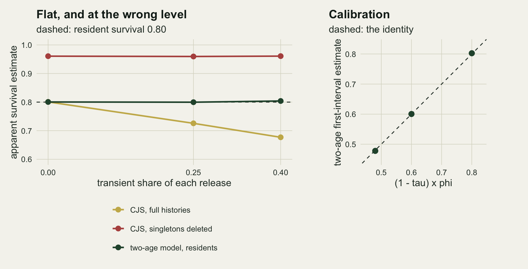
The deleted estimate follows survival, compressed
A flat line across transient shares says nothing about whether the rule can tell a good year from a bad one, because every point on it sits at the same true survival. The test that settles it varies the true resident survival instead, with no transients at all so that nothing but the rule is at work.
phi_grid <- c(0.55, 0.65, 0.80, 0.92)
set.seed(4417)
sweep_tab <- do.call(rbind, lapply(phi_grid, function(phi_i) {
  a <- run_cell(n_anchor, k_anchor, phi_i, p_anchor, 0)
  data.frame(phi = phi_i, full = mean(a[, "full"]), del = mean(a[, "del"]),
             tsm_two = mean(a[, "tsm_two"]), se_del = sd(a[, "del"]) / sqrt(n_anchor),
             del_lo = quantile(a[, "del"], 0.05), del_hi = quantile(a[, "del"], 0.95),
             tsm_lo = quantile(a[, "tsm_two"], 0.05), tsm_hi = quantile(a[, "tsm_two"], 0.95),
             pct_del = mean(a[, "pct_del"]))
}))
sweep_bias   <- sweep_tab$del - sweep_tab$phi
sweep_span   <- diff(range(sweep_tab$del))
truth_span   <- diff(range(phi_grid))
tsm_bias_max <- max(abs(sweep_tab$tsm_two - sweep_tab$phi))
The rule does follow survival. At true values of 0.55, 0.65, 0.80 and 0.92 the deleted arm reads 0.828, 0.885, 0.961 and 0.999, rising in step with the truth. What it does not do is follow it one for one. The bias is +0.278, +0.235, +0.161 and +0.079, largest where survival is lowest, and the estimate runs into the ceiling at one near the top. A span of 0.37 in true survival comes out as a span of 0.171 in the estimate. The two-age model on the same studies is never further than 0.005 from the truth.
The compression is the practical damage. A year in which a population loses almost half its adults and a year in which it loses a twelfth are the difference between a crash and a good season, and the deleted arm puts them 0.171 apart and reports both above 0.80. The deletion share moves the other way, from 67.6 per cent of marks at the lowest survival to 32.8 per cent at the highest, because a population with high mortality produces more birds that die before their second capture, and the rule removes exactly those.
sweep_long <- rbind(
  data.frame(phi = sweep_tab$phi, est = sweep_tab$del, lo = sweep_tab$del_lo,
             hi = sweep_tab$del_hi, arm = "CJS, singletons deleted"),
  data.frame(phi = sweep_tab$phi, est = sweep_tab$tsm_two, lo = sweep_tab$tsm_lo,
             hi = sweep_tab$tsm_hi, arm = "two-age model, residents"))

ggplot(sweep_long, aes(phi, est, colour = arm)) +
  geom_abline(slope = 1, intercept = 0, linetype = "dashed", colour = te_body, linewidth = 0.5) +
  geom_errorbar(aes(ymin = lo, ymax = hi), width = 0.012, linewidth = 0.5) +
  geom_line(linewidth = 0.9) +
  geom_point(size = 2.6) +
  scale_colour_manual(values = c(te_rust, te_forest), name = NULL) +
  scale_x_continuous(breaks = phi_grid) +
  coord_cartesian(xlim = c(0.5, 0.97), ylim = c(0.45, 1)) +
  labs(x = "true resident survival", y = "estimate",
       title = "Compressed against the ceiling",
       subtitle = "dashed: estimate equals truth; six occasions, detection 0.45") +
  theme_datasheet() +
  theme(legend.position = "bottom")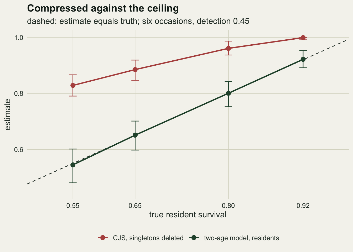
The survey design sets the level
The estimate after deletion is not a closed-form function of survival. It comes out of the joint likelihood, through a chi recursion that depends on survival, detection and the number of occasions together, so the design of the study enters the answer. The grid below crosses the four survival values with three detection probabilities and three study lengths, with a quarter of every release transient.
n_grid <- 150
p_grid <- c(0.25, 0.45, 0.70)
k_grid <- c(4, 6, 10)
design <- expand.grid(phi = phi_grid, p_det = p_grid, k_occ = k_grid)
set.seed(8123)
grid_tab <- do.call(rbind, lapply(seq_len(nrow(design)), function(i) {
  on_anchor <- design$phi[i] == phi_anchor
  a <- run_cell(n_grid, design$k_occ[i], design$phi[i], design$p_det[i], tau_anchor,
                gof = on_anchor)
  data.frame(design[i, ], del = mean(a[, "del"]), del_se = sd(a[, "del"]) / sqrt(n_grid),
             full = mean(a[, "full"]), tsm_two = mean(a[, "tsm_two"]),
             sec = mean(a[, "sec"]), pct_del = mean(a[, "pct_del"]),
             rej_chi = if (on_anchor) mean(a[, "chi"] > qchisq(0.95, a[, "df"])) else NA,
             rej_z = if (on_anchor) mean(a[, "z"] > qnorm(0.95)) else NA)
}))

cell <- function(ph, pp, kk) grid_tab[grid_tab$phi == ph & grid_tab$p_det == pp &
                                        grid_tab$k_occ == kk, ]
at_anchor  <- grid_tab[grid_tab$phi == phi_anchor, ]
del_p      <- sapply(p_grid, function(pp) cell(phi_anchor, pp, k_anchor)$del)
del_k      <- sapply(k_grid, function(kk) cell(phi_anchor, p_anchor, kk)$del)
design_min <- min(at_anchor$del); design_max <- max(at_anchor$del)
full_span  <- diff(range(at_anchor$full))
tsm_rng    <- range(at_anchor$tsm_two)
del_se_max <- max(grid_tab$del_se)
low_phi    <- grid_tab[grid_tab$phi == min(phi_grid), ]
high_phi   <- grid_tab[grid_tab$phi == max(phi_grid), ]
low_best   <- low_phi[which.max(low_phi$del), ]
high_worst <- high_phi[which.min(high_phi$del), ]
best_row   <- at_anchor[which.min(at_anchor$del), ]
bio_step   <- cell(phi_anchor, p_anchor, k_anchor)$del - cell(0.65, p_anchor, k_anchor)$del
Each of the 36 cells holds 150 studies. Hold survival at 0.80 and the transient share at 0.25, and the estimate after deletion reads 0.996, 0.960 and 0.914 at detection probabilities of 0.25, 0.45 and 0.70 over 6 occasions, and 1.000, 0.960 and 0.899 over 4, 6 and 10 occasions at detection 0.45. Across all nine designs at this one truth it runs from 0.874 to 1.000, a spread of 0.126. At the anchor design, raising the true survival from 0.65 to 0.80 moves the same estimate by 0.075. The largest Monte Carlo standard error of any cell mean in the grid is 0.0037, so none of these differences is noise. The two-age resident estimate across the same nine designs stays between 0.792 and 0.806.
The sharpest way to put it is to compare across truths. With true survival at 0.55, detection 0.25 and 4 occasions, the deleted arm reads 0.987. With true survival at 0.92, detection 0.70 and 10 occasions, it reads 0.949. A short, sparsely surveyed study of a population in a hard year returns a higher survival estimate than a long, well surveyed study of the same species in a good one. Two stations using the rule could rank their populations the wrong way round, and the ranking would say more about their net hours than about their birds.
The undeleted constant CJS also moves with the design, across 0.072 at this truth, because the weight the transients get in its blend depends on how many later captures the residents supply. That is the point of the joint live-dead post and is not the finding here. The rule does not remove the dependence on the survey; it trades a low blend for a high one that depends on the survey even more.
grid_plot <- grid_tab
grid_plot$k_lab <- factor(paste(grid_plot$k_occ, "occasions"),
                          levels = paste(k_grid, "occasions"))
grid_plot$p_lab <- factor(sprintf("detection %.2f", grid_plot$p_det),
                          levels = sprintf("detection %.2f", p_grid))

ggplot(grid_plot, aes(phi, del, colour = p_lab)) +
  geom_abline(slope = 1, intercept = 0, linetype = "dashed", colour = te_body, linewidth = 0.5) +
  geom_point(aes(y = tsm_two), shape = 4, size = 2, colour = te_body, stroke = 0.7) +
  geom_line(linewidth = 0.9) +
  geom_point(size = 2.2) +
  facet_wrap(~ k_lab, nrow = 1) +
  scale_colour_manual(values = c(te_gold, te_rust, te_ink), name = NULL) +
  scale_x_continuous(breaks = phi_grid) +
  coord_cartesian(ylim = c(0.5, 1)) +
  labs(x = "true resident survival", y = "estimate after deletion",
       title = "The survey sets the reading",
       subtitle = "crosses: two-age model on the undeleted data; dashed: estimate equals truth") +
  theme_datasheet() +
  theme(legend.position = "bottom",
        strip.text = element_text(colour = te_ink, face = "bold"),
        axis.text.x = element_text(size = 8))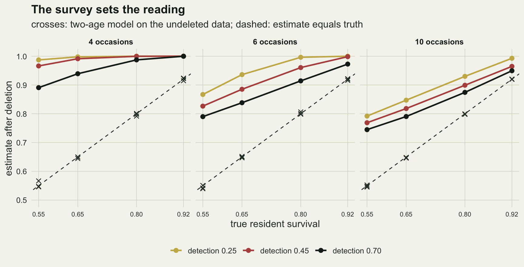
Under the most favourable design in the grid, 10 occasions at detection 0.70, the rule still overstates survival by 0.074, after deleting 46.7 per cent of the marks. More effort helps it; no design in this grid makes it right.
Where the damage sits
The rule reads the capture history to decide which birds stay, and the capture history is what the survival model is fitted to. Every bird that survives the rule has, by construction, been caught alive at least once after it was ringed. Its first interval, and every interval up to its second capture, is therefore survival that was guaranteed before the model saw it. The CJS likelihood is not told this. It treats the first release of each retained bird as an ordinary release, sees no deaths anywhere between release and second capture, and removes from the data the very animals whose chi terms carried the information about death.
That account makes a prediction. If the selection lives between the first capture and the second, then deleting the same birds but starting each history at its second capture should remove the bias, because nothing after the second capture was used to decide who stays. That is the third arm, the ad hoc approach of Pradel and colleagues, and it was computed in every study above.
sec_anchor <- anchor_tab$sec
sec_rng    <- range(at_anchor$sec)
sec_worst  <- at_anchor[which.max(abs(at_anchor$sec - phi_anchor)), ]
sec_other  <- sort(abs(at_anchor$sec - phi_anchor), decreasing = TRUE)[2]
sd_ratio   <- anchor_tab$sd_sec[2] / anchor_tab$sd_tsm[2]
At the anchor design it reads 0.803, 0.798 and 0.803 at the three transient shares, against a truth of 0.80, and across the nine designs of the grid at that truth it stays between 0.704 and 0.816. The low end of that range is the 4-occasion study at detection 0.25, where few birds reach a second capture and the fit rests on a small sample; in the other designs the arm is within 0.016 of the truth. Same birds, one capture fewer, and the bias of the rule is gone. The deletion was never the problem in itself; keeping the intervals that the deletion had already decided was the problem.
This arm is not offered as the repair. It discards every first capture along with every singleton, and at the anchor design, where every parameter is constant, its sampling standard deviation is 1.52 times that of the two-age resident estimate on the full data. The two-age model gets the same resident survival from the same likelihood, keeps the first interval as a parameter of its own, and throws nothing away.
Tight, and wrong
The deletion throws away 45.7 to 67.5 per cent of the marks at the anchor design, and the obvious expectation is that what survives the rule gives a much noisier estimate. The measurement says otherwise, and what it says is worse.
sd_ratio_del <- anchor_tab$sd_del / anchor_tab$sd_full
n_fail_all   <- sum(anchor_tab$n_fail)
quarter_runs <- anchor_runs[[2]]
del_cover    <- which(quarter_runs[, "del_lo"] <= phi_anchor & quarter_runs[, "del_hi"] >= phi_anchor)
cover_min_est <- min(quarter_runs[del_cover, "del"])
med_w_del    <- median(quarter_runs[, "del_hi"] - quarter_runs[, "del_lo"], na.rm = TRUE)
med_w_tsm    <- median(quarter_runs[, "tsm_hi"] - quarter_runs[, "tsm_lo"], na.rm = TRUE)
Across the 200 anchor studies with a quarter of the marks transient, the sampling standard deviation of the deleted estimate is 0.0194, against 0.0243 for the full CJS and 0.0307 for the two-age resident estimate: squeezed against the ceiling, the estimate has less room to vary, not more. Its Wald interval, built on the logit scale from the Hessian, has the same average width as the two-age interval to three decimals (0.120 against 0.120), but that average is carried by a few long intervals: the median width is 0.079 against 0.119. And the deleted interval contains the true 0.80 in 8.5 per cent of studies, against 96.0 per cent for the two-age model. The deleted intervals that do contain it all belong to studies whose estimate is pressed against one, at 0.988 or above, where the logit-scale interval stretches a long way down; they are the long intervals, not intervals centred near the truth.
At the other two transient shares the deleted interval covers the truth in 4.5 and 10.0 per cent of studies, and the two-age interval in 96.5 and 96.5 per cent. The full CJS covers 96.0 per cent with no transients present and 9.5 per cent with a quarter of them. Of the 2400 interval computations, 1 had a Hessian that could not be inverted; failures are left out of these rates.
n_show <- 40
tight_a <- anchor_runs[[2]][seq_len(n_show), ]
tight_df <- rbind(
  data.frame(est = tight_a[, "del"], lo = tight_a[, "del_lo"], hi = tight_a[, "del_hi"],
             arm = "CJS, singletons deleted"),
  data.frame(est = tight_a[, "tsm_two"], lo = tight_a[, "tsm_lo"], hi = tight_a[, "tsm_hi"],
             arm = "two-age model, residents"))
tight_df <- do.call(rbind, lapply(split(tight_df, tight_df$arm), function(d) {
  d <- d[order(d$est), ]
  d$rank <- seq_len(nrow(d))
  d$hits <- ifelse(d$lo <= phi_anchor & d$hi >= phi_anchor, "covers 0.80", "misses 0.80")
  d
}))

ggplot(tight_df, aes(x = est, y = rank, colour = hits)) +
  geom_vline(xintercept = phi_anchor, linetype = "dashed", colour = te_body, linewidth = 0.6) +
  geom_errorbar(aes(xmin = lo, xmax = hi), orientation = "y", width = 0, linewidth = 0.6) +
  geom_point(size = 1.6) +
  facet_wrap(~ arm, nrow = 1) +
  scale_colour_manual(values = c("covers 0.80" = te_forest, "misses 0.80" = te_rust),
                      name = NULL) +
  labs(x = "resident survival: estimate and 95 per cent Wald interval",
       y = "study, sorted by estimate",
       title = "An interval that rarely contains the truth",
       subtitle = "dashed: true resident survival") +
  theme_datasheet() +
  theme(legend.position = "bottom",
        strip.text = element_text(colour = te_ink, face = "bold"),
        axis.text.y = element_blank())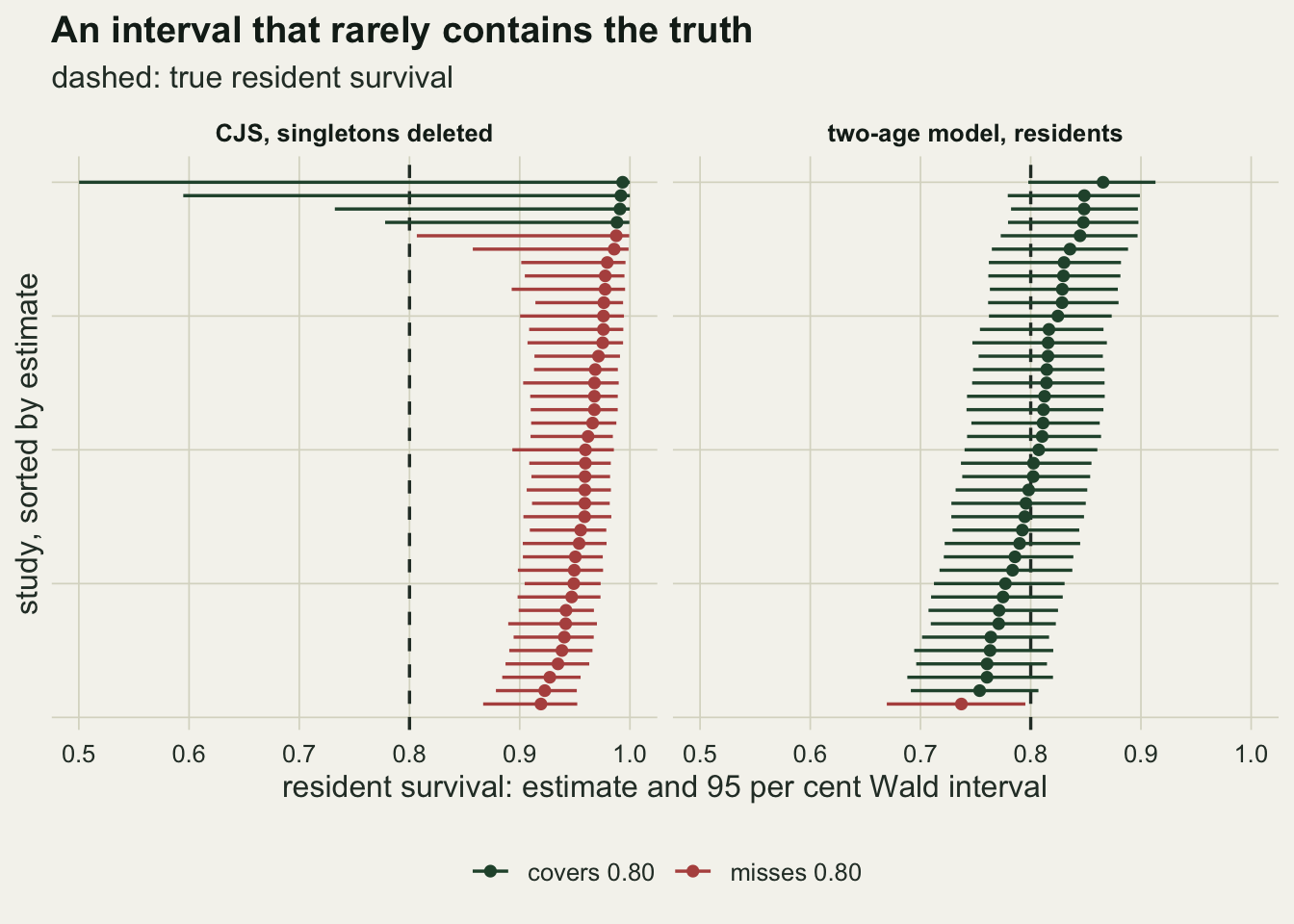
Test for transients instead of deleting them
The rule was a response to a real question: are there transients in these data? Pradel and colleagues pointed to TEST 3.SR, one of the standard components of CJS goodness of fit, as the component that answers it. At each occasion from the second to the second-last, take the birds caught there and split them into those ringed at that occasion and those ringed earlier. If there are no transients, the two groups should be equally likely to be seen again later. Transients are all in the first group and are never seen again, so a deficit of later sightings among the newly ringed birds is the signature. Each occasion gives a two by two table and a Pearson chi-square; the components are summed, with one degree of freedom each. The direction is recorded as a signed root of each component, positive when the previously ringed birds are more often seen again, and the signed roots are combined into a one-sided normal statistic by Stouffer’s method, which is the directional statistic for transience that U-CARE reports.
worked_3sr <- test_3sr(worked_sim$hist, worked_sim$first, k_anchor)
worked_p   <- pchisq(worked_3sr[["chi"]], worked_3sr[["df"]], lower.tail = FALSE)
mc_se_lvl  <- sqrt(0.05 * 0.95 / n_anchor)
pow_design <- at_anchor[order(at_anchor$k_occ, at_anchor$p_det), ]
weak_row   <- pow_design[which.min(pow_design$rej_chi), ]
In the worked study the summed statistic is 20.09 on 4 degrees of freedom, a p-value of 0.0005, and the directional statistic is 4.37.
Over the 200 anchor studies with no transients the summed test rejects at the five per cent level in 5.5 per cent of studies and the one-sided version in 5.0 per cent, where the Monte Carlo standard error of a five per cent rate is 1.5 percentage points. With a quarter of every release transient they reject in 78.0 and 97.5 per cent, and with two fifths in 99.5 and 100.0 per cent. The one-sided statistic is the better tool when the question is transients specifically, since transients can only push the tables one way.
The test has its own dependence on the design, and it is the honest kind: power rather than bias. At a quarter transient, the summed test rejects in 17.3 per cent of studies at 4 occasions and detection 0.25, the weakest design in the grid, and the one-sided version in 29.3 per cent. A short, sparse study may fail to detect transients that are there. It will not, as the deletion rule does, return a confident number that the design put there.
What to report
Report the TEST 3.SR result, both the summed chi-square with its degrees of freedom and the one-sided statistic, before any survival estimate. If it indicates transients, fit the two-age model and report the resident survival from the second parameter, with the first-interval estimate beside it. Name the second parameter for what a live-only model can estimate: apparent survival of residents, which is survival times fidelity, as the joint live-dead post shows. The first-interval parameter is survival times first-interval residency, and a transient and a bird that emigrates for good during its first interval are the same thing to it; the ratio of the two parameters is sometimes quoted as the proportion of residents among newly marked birds, and it carries that confound with it.
If a dataset has already been through a single-capture rule, say so, and state the number of occasions and the detection probability alongside the estimate, because across the designs measured above they move it further than a change in true survival from 0.65 to 0.80 does. If the original histories still exist, refit them.
State the deletion share with its denominator: all marks released, including those from the last release occasion, which are singletons far more often than the rest. A share quoted without that is not comparable between studies of different length.
Honest limits
The simulation is the textbook case for the two-age model. Transients leave at the moment of marking, residents share one constant survival and one constant detection, and every bird is an independent draw. Real transients may linger long enough to be caught at two occasions, and those birds pass the rule and stay in the data; the two-age model misreads them too, since it assumes transience is resolved in the first interval. Neither model here has time-dependent parameters. In a fully time-dependent two-age model the last parameters are confounded as in any CJS model, and nothing above checks how that interacts with the rule. The cost of the arm that restarts at the second capture, a standard deviation 1.52 times the two-age one, was measured with constant parameters only; with time-dependent survival and detection both models spend a parameter on every interval, and that comparison was not run.
The comparisons use one release size, 120 birds per occasion. The bias of the deleted arm comes from the selection rather than from sample size, so there is no reason to expect it to shrink with more birds, though only this one size was run. The small-sample behaviour of the arm that restarts at the second capture and the power of TEST 3.SR both depend on how many birds reach a second capture, and the weakest designs in the grid are where both are least reliable. The TEST 3.SR computed here uses Pearson chi-square on every table. U-CARE switches to Fisher’s exact test when expected counts are small, and the sparsest designs here are where that choice would matter.
The grid holds the transient share at a quarter, and for the deleted arm that choice matters only through sample size. Every transient here is a singleton, so the rule removes all of them, and what it keeps at a transient share tau is what it would keep from a study with no transients whose releases held only the residents, about (1 - tau) times as many birds. Another share would change the grid only through the number of residents, and the anchor runs, where the deleted estimate reads 0.961, 0.960 and 0.961 across the three shares, show how little that moves it.
TEST 3.SR compares newly marked birds with the rest, so anything that lowers survival or site fidelity in the first interval after marking produces the same signature as transience: a handling effect, or first-year birds ringed alongside adults. A significant result says the newly marked birds behave differently from the rest; transience is the usual reading, not the only one. Individual heterogeneity in detection among residents is not simulated here at all.
References
Pradel R, Hines JE, Lebreton JD, Nichols JD 1997 Biometrics 53(1):60-72 (10.2307/2533097)
Lebreton JD, Burnham KP, Clobert J, Anderson DR 1992 Ecological Monographs 62(1):67-118 (10.2307/2937171)
Choquet R, Lebreton JD, Gimenez O, Reboulet AM, Pradel R 2009 Ecography 32(6):1071-1074 (10.1111/j.1600-0587.2009.05968.x)