library(ggplot2)
library(patchwork)

te_paper  <- "#f5f4ee"
te_ink    <- "#16241d"
te_body   <- "#2c3a31"
te_forest <- "#275139"
te_rust   <- "#b5534e"
te_gold   <- "#c9b458"
te_line   <- "#dad9ca"

theme_datasheet <- function() {
  theme_minimal(base_size = 12) +
    theme(plot.background  = element_rect(fill = te_paper, colour = NA),
          panel.background = element_rect(fill = te_paper, colour = NA),
          panel.grid.major = element_line(colour = te_line, linewidth = 0.3),
          panel.grid.minor = element_blank(),
          text             = element_text(colour = te_body),
          plot.title       = element_text(colour = te_ink, face = "bold"),
          plot.subtitle    = element_text(colour = te_body),
          axis.text        = element_text(colour = te_body))
}Seed dispersal: the nearest adult is not the parent
R
seed dispersal
dispersal
spatial ecology
inverse modelling
simulation
ecology tutorial
Taking the nearest adult as the parent caps seed dispersal at the tree spacing. In R: that bias in closed form, and where the inverse seed-trap model fails.
A seedling census in a mapped forest plot gives two sets of coordinates: every adult of the species and every seedling under it. The quickest dispersal estimate from those two maps is to measure each seedling’s distance to the nearest adult of its own species, call that adult the parent, and fit a kernel to the distances. It needs no seed traps and no genotyping, and the same distance turns up as a covariate whenever a study asks how far a recruit is from its parent.
The trouble with it is known. Nathan and Muller-Landau’s review of seed dispersal patterns points out that the nearest adult is an assumption about parentage, not an observation of it, and Hardesty, Hubbell and Bermingham genotyped the recruits of a vertebrate-dispersed tree and found frequent long-distance recruitment, with seedlings coming from mothers well beyond the nearest adult. The standard way round it without genetics is the inverse model of Ribbens, Silander and Pacala, carried over to seed traps by Clark and colleagues: predict the seed rain at each point as the sum of the kernel over every adult in the stand, and fit the kernel to the counts. This post is a demonstration of that literature, not a claim to it. What it adds is narrower. How wrong the shortcut is follows from one dimensionless number that can be computed before fieldwork, and it follows by formula, so the first half of the post is a derivation checked by simulation rather than a simulation result. The second half is measured: where the inverse model itself, fed a few seeds per trap, stops identifying the kernel, and what does and does not fix that.
The kernel posts on this site all measure distance from a source they know. Fitting dispersal kernels in R fits the distance density of the two-dimensional exponential kernel to distances from a known tree, and the same kernel is used below. Checking a dispersal kernel deals with a trap window of fixed radius around that tree, a cap on distance that the analyst chose. Here the source is the unknown and the cap is not chosen: it is the random spacing between adults, whose expected value Plotless density estimation from distances derives as 1 / (2 * sqrt(lambda)). Misread rings and the dispersal tail follows a different wrong-partner error, in which a misread ring joins a recovery to a random ringing site anywhere in the scheme and fattens the tail. The nearest adult is the opposite kind of wrong partner, the closest one available, and it shrinks the distances. The same distance is also the axis of Janzen-Connell and tree diversity, which calls its own model a one-tree model; a field test of that model that measures distance to the nearest conspecific adult inherits the cap below.
The shortcut, done with a pencil
Take adults scattered at random, a Poisson pattern with density lambda per square metre, and a seedling that landed a distance R from its true parent. By Slivnyak’s theorem, if one adult of a Poisson pattern is known to stand at a given place, the others are still a Poisson pattern of the same density; the seedling’s position is that adult’s position plus an independent dispersal step, so the other adults seen from the seedling are Poisson too, whatever R is. It is the property the plotless estimators lean on. So the distance D from the seedling to the nearest other adult has P(D > r) = exp(-lambda * pi * r^2), the empty-disc probability, and it is independent of R. The shortcut records min(R, D) and names the wrong adult whenever D < R. Two lines follow:
\[ P(\text{wrong}) = P(D < R) = 1 - E\left[e^{-\lambda \pi R^2}\right], \qquad E[\min(R, D)] = \int_0^\infty P(R > r)\, e^{-\lambda \pi r^2}\, dr . \]
For the two-dimensional exponential kernel the distance R has a Gamma distribution with shape 2 and scale a, mean mu = 2 a, so P(R > r) = (1 + r / a) exp(-r / a). Measure every distance in units of the expected nearest-neighbour spacing 0.5 / sqrt(lambda) and the density drops out of both integrals: lambda * pi * r^2 becomes pi * r^2 / 4, and the kernel enters only through its mean in those units,
\[ \kappa = \frac{\mu}{0.5 / \sqrt{\lambda}} = 2 \mu \sqrt{\lambda} . \]
Kappa is the reach of the kernel in adult spacings. A stand map gives lambda, a guess at the mean dispersal distance gives mu, and the number is ready before a single seedling is measured. Because min(R, D) can never exceed D, the assigned mean distance can never exceed the spacing, so the ratio of assigned to true mean distance is capped by 1 / kappa at every kappa, not only in a limit. Unequal fecundity does not change the argument: the parent is then a pick weighted by fecundity, but the other adults are still a Poisson pattern around the seedling.
kappa_of <- function(dens_ha, mu) 2 * mu * sqrt(dens_ha / 1e4)

# distances in units of the expected nearest-neighbour spacing 0.5 / sqrt(lambda),
# so lambda * pi * r^2 becomes pi * r^2 / 4 and the kernel mean is kappa itself
shortcut_cf <- function(kappa) {
  a <- kappa / 2
  empty_disc <- function(r) exp(-pi * r^2 / 4)
  wrong <- 1 - integrate(function(r) dgamma(r, 2, scale = a) * empty_disc(r),
                         0, Inf)$value
  mean_nn <- integrate(function(r) (1 + r / a) * exp(-r / a) * empty_disc(r),
                       0, Inf)$value
  c(kappa = kappa, ratio = mean_nn / kappa, wrong = wrong)
}

cf_curve <- as.data.frame(t(sapply(exp(seq(log(0.2), log(8), length.out = 150)),
                                   shortcut_cf)))
kappa_half_wrong <- uniroot(function(k) shortcut_cf(k)[["wrong"]] - 0.5,
                            c(0.2, 8))$root
kappa_half_ratio <- uniroot(function(k) shortcut_cf(k)[["ratio"]] - 0.5,
                            c(0.2, 8))$root
spacing_20 <- 0.5 / sqrt(20 / 1e4)
cf_gravity <- shortcut_cf(kappa_of(20, 5))
cf_wind30 <- shortcut_cf(kappa_of(20, 30))
cf_wind60 <- shortcut_cf(kappa_of(20, 60))
cap_gap30 <- 1 - cf_wind30[["ratio"]] * cf_wind30[["kappa"]]
print(round(rbind(gravity = cf_gravity, wind30 = cf_wind30, wind60 = cf_wind60), 3))
kappa ratio wrong
gravity 0.447 0.881 0.174
wind30 2.683 0.336 0.820
wind60 5.367 0.180 0.938print(round(c(kappa_half_wrong = kappa_half_wrong,
kappa_half_ratio = kappa_half_ratio), 3))kappa_half_wrong kappa_half_ratio
1.087 1.596 Two integrate() calls are the whole method. The wrong-parent share passes one half at kappa 1.09, and the assigned mean distance falls to half the true one at kappa 1.60. A short, gravity-dispersed kernel is not safe either: 20 adults per hectare with a mean dispersal distance of 5 m is kappa 0.45, and the formula assigns 17 per cent of seedlings to the wrong adult, although their distances survive fairly well (ratio 0.88). At 20 adults per hectare the spacing is 11.2 m, so a wind-dispersed kernel with a 30 m mean sits at kappa 2.68: the ratio is 0.336 against a cap of 0.373, only 10 per cent below it, and at a 60 m mean it is 0.180 against 0.186. From kappa of about two upwards the nearest-adult distance measures the stand, not the seed, and a kernel fitted to it inherits the stand’s spacing as its scale.
A simulated stand as the check
A formula derived this way can still hide a slip, so it is checked against the generator used for the rest of the post: a 600 x 600 m stand, adults placed at random, each adult shedding seeds with Gamma-distributed distances and uniform directions, and every seedling that lands in the central 200 x 200 m window measured to every adult. The window keeps seedlings at least 200 m from the stand edge, so no seedling misses a nearer adult standing off the map. Seed output is proportional to the number of adults, so a stand with more adults near the window contributes more seedlings, which is the weighting the formula assumes. The cells run from an animal-dispersed tropical tree at 2 adults per hectare to a dominant canopy tree at 100, and include a pair that shares one kappa from two different stands (20 per hectare at 30 m and 80 per hectare at 15 m) and two arms outside the formula’s assumptions: Thomas-clustered adults and lognormal fecundity.
stand_side <- 600
core <- c(200, 400)

place_adults <- function(dens_ha, pattern = "poisson") {
  n_ad <- rpois(1, dens_ha * stand_side^2 / 1e4)
  if (pattern == "poisson")
    return(cbind(runif(n_ad, 0, stand_side), runif(n_ad, 0, stand_side)))
  # Thomas process: parents at a quarter of the adult density, adults
  # scattered around them with sd 15 m, wrapped on a torus
  n_par <- max(1, rpois(1, n_ad / 4))
  par_xy <- cbind(runif(n_par, 0, stand_side), runif(n_par, 0, stand_side))
  pick <- sample.int(n_par, n_ad, replace = TRUE)
  (par_xy[pick, , drop = FALSE] + matrix(rnorm(2 * n_ad, 0, 15), n_ad)) %% stand_side
}

shortcut_draw <- function(dens_ha, mu, pattern = "poisson", fec_sd = 0) {
  a <- mu / 2
  adults <- place_adults(dens_ha, pattern)
  fec <- exp(rnorm(nrow(adults), 0, fec_sd))
  # seed output proportional to the number of adults, so a stand with more
  # adults near the core contributes more seedlings, as it would in the field;
  # about 400 of them land in the central 200 x 200 m window
  n_cand <- round(100 * nrow(adults) / dens_ha)
  parent <- sample.int(nrow(adults), n_cand, replace = TRUE, prob = fec)
  step_r <- rgamma(n_cand, 2, scale = a)
  angle <- runif(n_cand, 0, 2 * pi)
  sx <- adults[parent, 1] + step_r * cos(angle)
  sy <- adults[parent, 2] + step_r * sin(angle)
  keep <- which(sx > core[1] & sx < core[2] & sy > core[1] & sy < core[2])
  d2 <- outer(sx[keep], adults[, 1], "-")^2 + outer(sy[keep], adults[, 2], "-")^2
  nearest <- max.col(-d2, ties.method = "first")
  d_nn <- sqrt(d2[cbind(seq_along(keep), nearest)])
  c(n = length(keep), sum_nn = sum(d_nn), sum_true = sum(step_r[keep]),
    n_wrong = sum(nearest != parent[keep]))
}

# pooled over draws: ratio of summed distances, share of all seedlings
pool_draws <- function(draws) {
  n <- draws["n", ]; tt <- draws["sum_true", ]; nn <- draws["sum_nn", ]
  w <- draws["n_wrong", ]; k <- ncol(draws)
  ratio <- sum(nn) / sum(tt); wrong <- sum(w) / sum(n)
  c(ratio = ratio, ratio_se = sd(nn - ratio * tt) / (mean(tt) * sqrt(k)),
    wrong = wrong, wrong_se = sd(w - wrong * n) / (mean(n) * sqrt(k)),
    per_draw = mean(n))
}

shortcut_cells <- data.frame(
  dens = c(2, 5, 20, 20, 20, 100, 80, 20, 20),
  mu = c(40, 30, 5, 30, 60, 10, 15, 30, 30),
  pattern = c(rep("poisson", 7), "thomas", "poisson"),
  fec_sd = c(rep(0, 8), 1),
  arm = c(rep("Poisson adults", 7), "Thomas clustered adults", "Unequal fecundity"))
n_draw_short <- 100

set.seed(3271)
short_tab <- do.call(rbind, lapply(seq_len(nrow(shortcut_cells)), function(i) {
  cc <- shortcut_cells[i, ]
  pooled <- pool_draws(replicate(n_draw_short,
                                 shortcut_draw(cc$dens, cc$mu, cc$pattern, cc$fec_sd)))
  cf <- shortcut_cf(kappa_of(cc$dens, cc$mu))
  data.frame(cc, kappa = cf[["kappa"]],
             ratio_sim = pooled[["ratio"]], ratio_se = pooled[["ratio_se"]],
             ratio_cf = cf[["ratio"]], one_over_kappa = 1 / cf[["kappa"]],
             wrong_sim = pooled[["wrong"]], wrong_se = pooled[["wrong_se"]],
             wrong_cf = cf[["wrong"]], per_draw = pooled[["per_draw"]])
}))
short_tab$z_ratio <- (short_tab$ratio_sim - short_tab$ratio_cf) / short_tab$ratio_se
short_tab$z_wrong <- (short_tab$wrong_sim - short_tab$wrong_cf) / short_tab$wrong_se
print(format(short_tab[, c("dens", "mu", "arm", "kappa", "ratio_sim", "ratio_cf",
                           "one_over_kappa", "wrong_sim", "wrong_cf", "z_ratio",
                           "z_wrong", "per_draw")], digits = 3),
      row.names = FALSE)
dens mu arm kappa ratio_sim ratio_cf one_over_kappa
2 40 Poisson adults 1.131 0.617 0.620 0.884
5 30 Poisson adults 1.342 0.562 0.560 0.745
20 5 Poisson adults 0.447 0.876 0.881 2.236
20 30 Poisson adults 2.683 0.334 0.336 0.373
20 60 Poisson adults 5.367 0.182 0.180 0.186
100 10 Poisson adults 2.000 0.425 0.424 0.500
80 15 Poisson adults 2.683 0.336 0.336 0.373
20 30 Thomas clustered adults 2.683 0.345 0.336 0.373
20 30 Unequal fecundity 2.683 0.334 0.336 0.373
wrong_sim wrong_cf z_ratio z_wrong per_draw
0.529 0.517 -0.549 1.8527 409
0.582 0.588 0.375 -1.0855 397
0.179 0.174 -2.531 1.9210 403
0.821 0.820 -0.592 0.4632 406
0.937 0.938 1.218 -0.8949 397
0.733 0.735 0.524 -1.0550 399
0.820 0.820 0.545 0.0333 400
0.840 0.820 2.702 6.8622 410
0.821 0.820 -0.834 0.4528 397pois_rows <- short_tab[short_tab$arm == "Poisson adults", ]
max_abs_z <- max(abs(c(pois_rows$z_ratio, pois_rows$z_wrong)))
pair_a <- short_tab[short_tab$dens == 20 & short_tab$mu == 30 &
short_tab$arm == "Poisson adults", ]
pair_b <- short_tab[short_tab$dens == 80 & short_tab$mu == 15, ]
thomas_row <- short_tab[short_tab$arm == "Thomas clustered adults", ]
fec_row <- short_tab[short_tab$arm == "Unequal fecundity", ]
n_compare <- 2 * nrow(pois_rows)
mean_per_draw <- mean(short_tab$per_draw)Over 100 stands per cell, about 402 seedlings each, the simulated points sit on the formula. Across the seven Poisson cells the largest gap is 2.5 Monte Carlo standard errors, in 14 comparisons. The collapse pair gives ratios of 0.334 and 0.336 and wrong shares of 0.821 and 0.820: a stand four times as dense with a kernel half as long is the same problem. Lognormal fecundity (sdlog 1) gives 0.334 and 0.821 against the formula’s 0.336 and 0.820, as the argument above says it should. Clustering barely matters: Thomas-clustered adults move the ratio to 0.345 and the wrong share to 0.840, a shift this replication can detect but not one that changes the reading. None of this is a finding. The points are there to show that the pencil was right.
arm_shapes <- c("Poisson adults" = 21, "Thomas clustered adults" = 22,
                "Unequal fecundity" = 24)
arm_fills <- c("Poisson adults" = te_forest, "Thomas clustered adults" = te_gold,
               "Unequal fecundity" = te_rust)
asym <- data.frame(kappa = cf_curve$kappa[cf_curve$kappa >= 0.8])
p_ratio <- ggplot(cf_curve, aes(kappa, ratio)) +
  geom_line(data = asym, aes(kappa, 1 / kappa), linetype = 2, colour = te_body,
            linewidth = 0.4) +
  geom_line(colour = te_ink, linewidth = 0.8) +
  geom_point(data = short_tab, aes(kappa, ratio_sim, shape = arm, fill = arm),
             size = 2.6, colour = te_ink, stroke = 0.4) +
  annotate("text", x = 3.6, y = 0.38, label = "1 / kappa", colour = te_body,
           hjust = 0, size = 3.6) +
  scale_x_log10(breaks = c(0.2, 0.5, 1, 2, 5)) +
  scale_shape_manual(values = arm_shapes, name = NULL) +
  scale_fill_manual(values = arm_fills, name = NULL) +
  labs(x = "kappa = mean dispersal distance / spacing",
       y = "Nearest-adult / true mean distance", title = "Distance kept") +
  theme_datasheet() + theme(legend.position = "bottom")
p_wrong <- ggplot(cf_curve, aes(kappa, wrong)) +
  geom_line(colour = te_ink, linewidth = 0.8) +
  geom_point(data = short_tab, aes(kappa, wrong_sim, shape = arm, fill = arm),
             size = 2.6, colour = te_ink, stroke = 0.4) +
  scale_x_log10(breaks = c(0.2, 0.5, 1, 2, 5)) +
  scale_y_continuous(limits = c(0, 1)) +
  scale_shape_manual(values = arm_shapes, name = NULL) +
  scale_fill_manual(values = arm_fills, name = NULL) +
  labs(x = "kappa = mean dispersal distance / spacing",
       y = "Share assigned to the wrong parent", title = "Wrong parent") +
  theme_datasheet() + theme(legend.position = "bottom")
(p_ratio | p_wrong) +
  plot_layout(guides = "collect") +
  plot_annotation(theme = theme_datasheet()) &
  theme(legend.position = "bottom")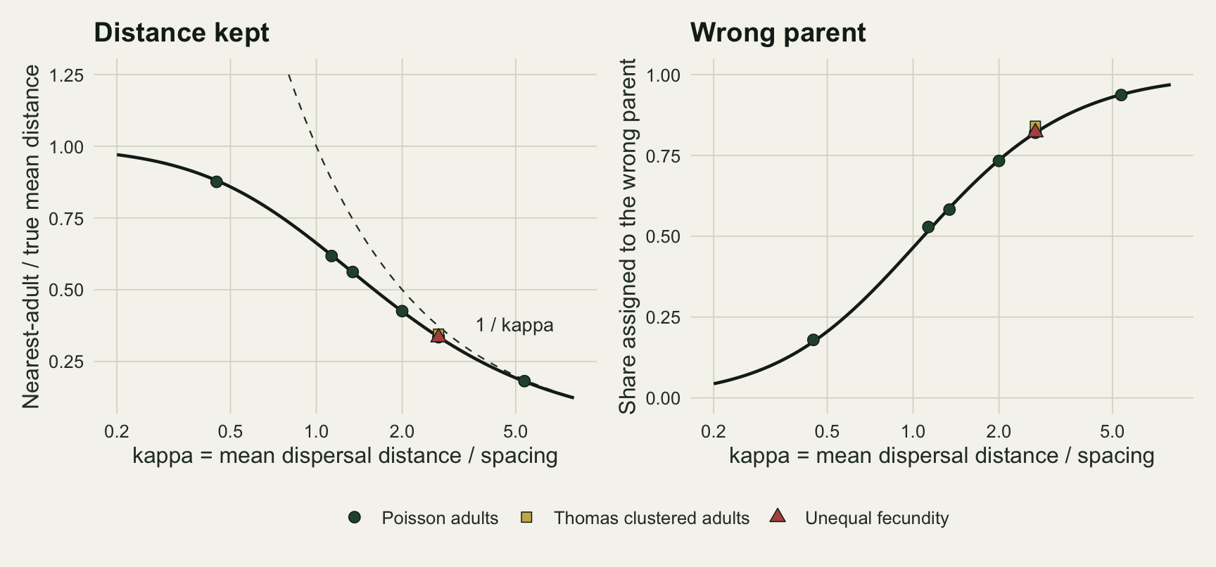
The inverse model: sum over every adult
The inverse model takes the other route. Instead of asking which adult produced each seedling, it predicts the seed rain at each trap as the sum of the kernel over every adult in the stand, weighted by fecundity, and fits the kernel scale to the counts. Nothing is capped by the nearest neighbour, because every adult contributes to every trap. The version here follows Ribbens and colleagues in summing over mapped adults and Clark and colleagues in fitting trap counts: a 10 x 10 grid of 0.5 square metre traps centred in the stand, a mean output of 3000 seeds per adult, Poisson counts, the correct kernel family and every adult position known exactly. Fecundity is a nuisance parameter. Given the scale, its maximum-likelihood value is the total catch over the total predicted rain, so it is profiled out and the scale is found by a one-dimensional search between 1 and 400 m. That is a generous version of the method: real trap data add overdispersion, doubt about the kernel family and unmapped adults beyond the plot edge.
kernel2d <- function(r, a) exp(-r / a) / (2 * pi * a^2)
trap_area <- 0.5
seeds_per_adult <- 3000
a_bounds <- c(1, 400)

trap_data <- function(dens_ha, mu, extent, pattern = "poisson", fec_sd = 0,
                      seeds = seeds_per_adult, n_side = 10) {
  adults <- place_adults(dens_ha, pattern)
  fec <- exp(rnorm(nrow(adults), 0, fec_sd))
  fec <- fec / mean(fec)
  g <- seq(stand_side / 2 - extent / 2, stand_side / 2 + extent / 2, length.out = n_side)
  traps <- as.matrix(expand.grid(g, g))
  dist <- sqrt(outer(traps[, 1], adults[, 1], "-")^2 +
               outer(traps[, 2], adults[, 2], "-")^2)
  y <- rpois(nrow(traps), seeds * trap_area * as.vector(kernel2d(dist, mu / 2) %*% fec))
  list(y = y, dist = dist)
}

# Poisson likelihood of the trap counts; fecundity F profiled out (its MLE given
# the scale is sum(y) / sum(K)), unless it is supplied as known
scale_nll <- function(log_a, y, dist, known_F = NA) {
  K <- trap_area * rowSums(kernel2d(dist, exp(log_a)))
  F_hat <- if (is.na(known_F)) sum(y) / sum(K) else known_F
  -sum(dpois(y, F_hat * K, log = TRUE))
}

fit_scale <- function(td, known_F = NA, interval = FALSE) {
  opt <- optimize(scale_nll, log(a_bounds), y = td$y, dist = td$dist, known_F = known_F)
  out <- c(a_hat = exp(opt$minimum), lo = NA, hi = NA)
  if (interval) {
    cut_nll <- opt$objective + qchisq(0.95, 1) / 2
    gap <- function(la) scale_nll(la, td$y, td$dist, known_F) - cut_nll
    out[["lo"]] <- if (gap(log(a_bounds[1])) > 0)
      exp(uniroot(gap, c(log(a_bounds[1]), opt$minimum))$root) else a_bounds[1]
    out[["hi"]] <- if (gap(log(a_bounds[2])) > 0)
      exp(uniroot(gap, c(opt$minimum, log(a_bounds[2])))$root) else a_bounds[2]
  }
  out
}

run_cell <- function(n_rep, dens_ha, mu, extent, pattern = "poisson", fec_sd = 0,
                     seeds = seeds_per_adult, n_side = 10, known = FALSE,
                     interval = FALSE) {
  a <- mu / 2
  res <- replicate(n_rep, {
    td <- trap_data(dens_ha, mu, extent, pattern, fec_sd, seeds, n_side)
    f <- fit_scale(td, known_F = if (known) seeds else NA, interval = interval)
    c(f, seeds_trap = mean(td$y))
  })
  ratio <- res["a_hat", ] / a
  data.frame(dens = dens_ha, mu = mu, kappa = kappa_of(dens_ha, mu), extent = extent,
             median = median(ratio), q25 = quantile(ratio, 0.25),
             q75 = quantile(ratio, 0.75),
             fail = mean(ratio > 1.5 | ratio < 1 / 1.5),
             hi = mean(ratio > 1.5), lo = mean(ratio < 1 / 1.5),
             mean_ratio = mean(ratio),
             at_bound = mean(res["a_hat", ] > 0.99 * a_bounds[2]),
             seeds_trap = mean(res["seeds_trap", ]),
             width = if (interval) median(res["hi", ] / res["lo", ]) else NA,
             cover = if (interval) mean(res["lo", ] <= a & res["hi", ] >= a) else NA,
             row.names = NULL)
}
Before any fitting it helps to look at what the traps are being shown. The map below is the expected seed rain relative to its mean over a 180 m square, for one stand at 20 adults per hectare, under a 15 m and a 60 m mean dispersal distance.
set.seed(3272)
rain_stand <- place_adults(20)
px <- seq(210, 390, length.out = 91)
pix <- as.matrix(expand.grid(px, px))
pix_dist <- sqrt(outer(pix[, 1], rain_stand[, 1], "-")^2 +
                 outer(pix[, 2], rain_stand[, 2], "-")^2)
rain_map <- do.call(rbind, lapply(c(15, 60), function(mu) {
  expct <- rowSums(kernel2d(pix_dist, mu / 2))
  data.frame(x = pix[, 1], y = pix[, 2], rel = expct / mean(expct),
             panel = sprintf("mean distance %d m, kappa %.1f", mu, kappa_of(20, mu)))
}))
rain_ad <- as.data.frame(rain_stand)
names(rain_ad) <- c("x", "y")
rain_ad <- rain_ad[rain_ad$x > 210 & rain_ad$x < 390 & rain_ad$y > 210 & rain_ad$y < 390, ]

mu_grid <- c(15, 30, 45, 60)
cv_signal <- sapply(mu_grid, function(mu) mean(replicate(50, {
  td <- trap_data(20, mu, 180)
  lam <- rowSums(kernel2d(td$dist, mu / 2))
  sd(lam) / mean(lam)
})))
seeds_trap_20 <- seeds_per_adult * trap_area * 20 / 1e4
cv_noise <- 1 / sqrt(seeds_trap_20)
sig_noise_wide <- cv_signal[4] / cv_noise
print(round(c(setNames(cv_signal, sprintf("mu%d", mu_grid)), noise = cv_noise), 3))
mu15 mu30 mu45 mu60 noise
0.573 0.280 0.175 0.118 0.577 ggplot(rain_map, aes(x, y, fill = pmin(pmax(log2(rel), -3), 3))) +
geom_raster() +
geom_point(data = rain_ad, aes(x, y), inherit.aes = FALSE, shape = 21,
fill = te_paper, colour = te_ink, size = 1.4) +
facet_wrap(~ panel) +
scale_fill_gradient2(low = te_forest, mid = te_paper, high = te_rust, midpoint = 0,
limits = c(-3, 3), breaks = -3:3,
labels = c("1/8", "1/4", "1/2", "1", "2", "4", "8"),
name = "Expected rain /\nits mean") +
coord_equal(expand = FALSE) +
labs(x = "Easting (m)", y = "Northing (m)") +
theme_datasheet() +
theme(strip.text = element_text(colour = te_ink, face = "bold"))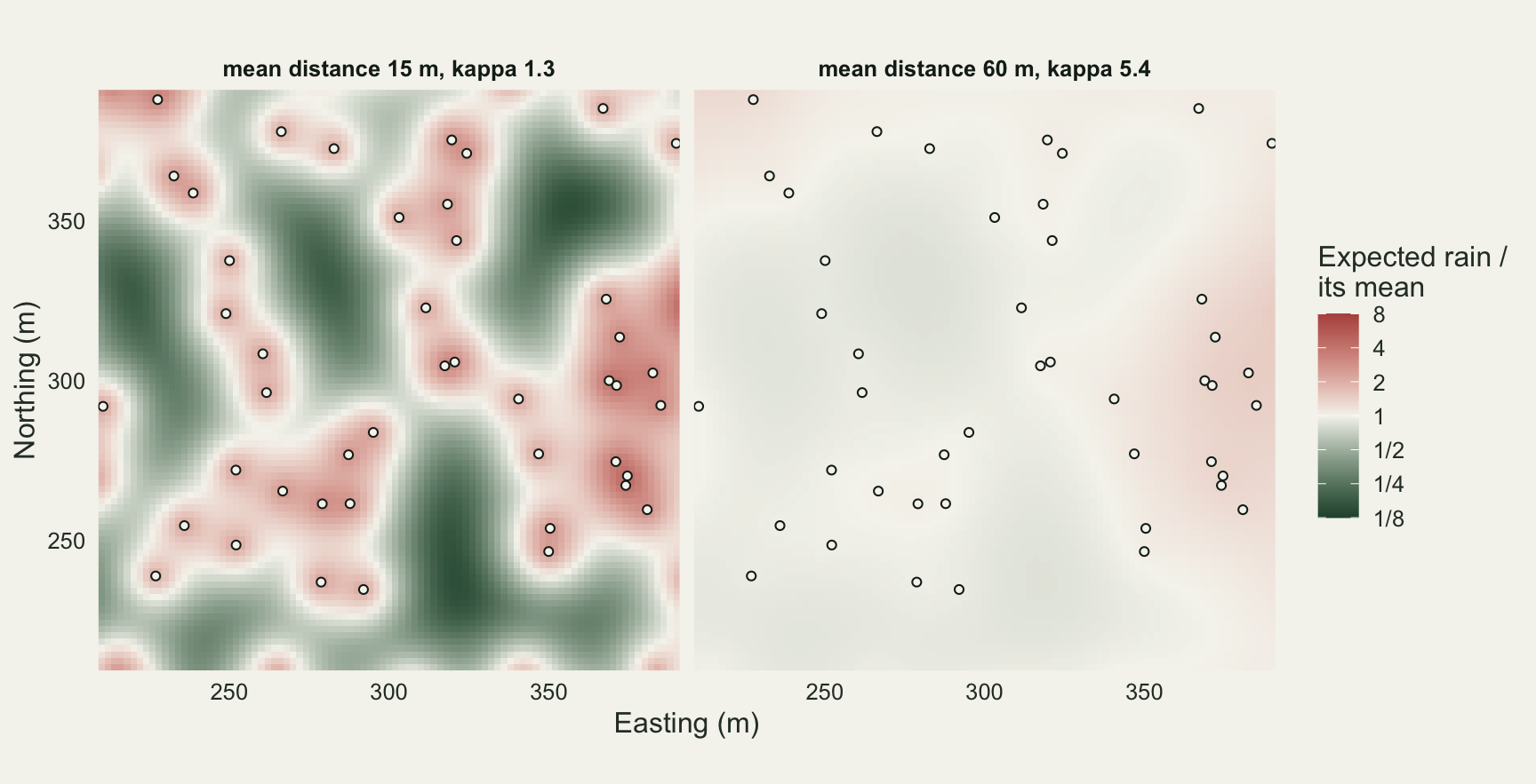
At kappa 1.3 the rain is a relief map of the adults: several times the mean under each tree, a fraction of it in the gaps. At kappa 5.4 the same adults produce a gentle slope. The scale of the kernel is written in that relief and nowhere else, because the total catch is set by fecundity times density whatever the scale is. Averaged over 50 stands, the coefficient of variation of the expected rain across the 100 trap positions of the 180 m grid is 0.57 at kappa 1.3, 0.28 at 2.7, 0.18 at 4.0 and 0.12 at 5.4, while Poisson counting noise at 3 seeds per trap has a coefficient of variation of 0.58. At the short kernel the differences between traps are as large as the counting noise; at the widest they are 0.20 of it.
Where the repair loses the scale
The sweep holds the stand at 20 adults per hectare and the trap count at 100, and varies the mean dispersal distance (15, 30, 45 and 60 m, kappa from 1.3 to 5.4) and the side of the square trap grid (90, 180 and 360 m, so trap spacing grows with the grid). Each cell is 200 simulated data sets, and the failure share is counted over data sets, never over traps or seeds: the share whose fitted scale is off by more than a factor of 1.5 in either direction. The profile-likelihood interval of the next section is computed for every data set on the 180 m grid.
n_rep_inv <- 200
ext_grid <- c(90, 180, 360)
set.seed(3273)
sweep_tab <- do.call(rbind, lapply(mu_grid, function(mu)
  do.call(rbind, lapply(ext_grid, function(ext)
    run_cell(n_rep_inv, 20, mu, ext, interval = (ext == 180))))))
sweep_tab$fail_se <- sqrt(sweep_tab$fail * (1 - sweep_tab$fail) / n_rep_inv)
print(format(sweep_tab[, c("mu", "kappa", "extent", "median", "q25", "q75", "fail",
                           "hi", "lo", "mean_ratio", "fail_se", "at_bound",
                           "seeds_trap")], digits = 3),
      row.names = FALSE)
mu kappa extent median q25 q75 fail hi lo mean_ratio fail_se
15 1.34 90 1.004 0.941 1.06 0.000 0.000 0.000 1.007 0.00000
15 1.34 180 0.994 0.934 1.05 0.000 0.000 0.000 0.998 0.00000
15 1.34 360 1.005 0.951 1.06 0.005 0.005 0.000 1.008 0.00499
30 2.68 90 0.983 0.903 1.14 0.045 0.045 0.000 1.245 0.01466
30 2.68 180 0.972 0.879 1.12 0.050 0.050 0.000 1.029 0.01541
30 2.68 360 0.992 0.887 1.10 0.065 0.065 0.000 1.079 0.01743
45 4.02 90 1.000 0.847 1.23 0.165 0.150 0.015 1.905 0.02625
45 4.02 180 0.970 0.873 1.16 0.135 0.105 0.030 1.230 0.02416
45 4.02 360 0.983 0.853 1.16 0.125 0.095 0.030 1.118 0.02339
60 5.37 90 1.009 0.780 1.39 0.295 0.215 0.080 2.222 0.03225
60 5.37 180 1.024 0.839 1.35 0.245 0.190 0.055 1.707 0.03041
60 5.37 360 0.992 0.790 1.28 0.235 0.150 0.085 1.203 0.02998
at_bound seeds_trap
0.000 3.05
0.000 3.01
0.000 2.99
0.005 2.99
0.000 3.02
0.000 2.99
0.035 3.03
0.005 3.04
0.000 2.99
0.075 2.98
0.035 3.00
0.000 2.97cell_of <- function(mu, ext) sweep_tab[sweep_tab$mu == mu & sweep_tab$extent == ext, ]
wide_rows <- sweep_tab[sweep_tab$mu == 60, ]
mid_rows <- sweep_tab[sweep_tab$mu == 30, ]
k4_rows <- sweep_tab[sweep_tab$mu == 45, ]
short_rows <- sweep_tab[sweep_tab$mu == 15, ]
ext_gap <- cell_of(60, 90)$fail - cell_of(60, 360)$fail
ext_gap_se <- sqrt(cell_of(60, 90)$fail_se^2 + cell_of(60, 360)$fail_se^2)At kappa 1.3 the inverse model is as good as exact: at most 0.005 of data sets are off by 1.5x on any grid. At kappa 2.7 the failure share is 0.045 to 0.065, at 4.0 it is 0.125 to 0.165, and at 5.4 it is 0.235 to 0.295 across the three grids, with Monte Carlo standard errors of about 0.03. The median fitted-to-true ratio stays between 0.97 and 1.02 in every cell, so the typical fit is on target. At the widest kernel the failures run mostly in the long direction: on the 90, 180 and 360 m grids 0.215, 0.190 and 0.150 of data sets give a scale more than 1.5 times too wide, against 0.080, 0.055 and 0.085 more than 1.5 times too narrow. The long misses are large enough to drag the mean with them: the mean fitted-to-true ratio at kappa 5.4 is 2.22, 1.71 and 1.20 on the three grids, so the estimator is median-unbiased but not mean-unbiased. Mean seeds per trap is 2.97 to 3.05 in every cell of the sweep, so the rise is not a sparse-rain effect: the traps catch as many seeds at kappa 1.3 as at 5.4, and those seeds say less. At kappa 5.4 a share of the fits runs to the top of the search interval, 0.075 on the 90 m grid, 0.035 on the 180 m grid and 0.000 on the 360 m grid: there the likelihood prefers a rain with no relief at all.
sweep_tab$grid <- factor(sprintf("%d m grid", sweep_tab$extent),
                         levels = sprintf("%d m grid", ext_grid))
ext_cols <- setNames(c(te_gold, te_forest, te_rust), levels(sweep_tab$grid))
ggplot(sweep_tab, aes(kappa, fail, colour = grid)) +
  geom_hline(yintercept = 0, colour = te_line) +
  geom_line(linewidth = 0.8) +
  geom_errorbar(aes(ymin = pmax(fail - 2 * fail_se, 0), ymax = fail + 2 * fail_se),
                width = 0.08, linewidth = 0.5) +
  geom_point(size = 2.4) +
  scale_colour_manual(values = ext_cols, name = NULL) +
  labs(x = "kappa = mean dispersal distance / spacing",
       y = "Share of data sets off by more than 1.5x",
       title = "The inverse model fails where the shortcut is worst") +
  theme_datasheet() + theme(legend.position = "bottom")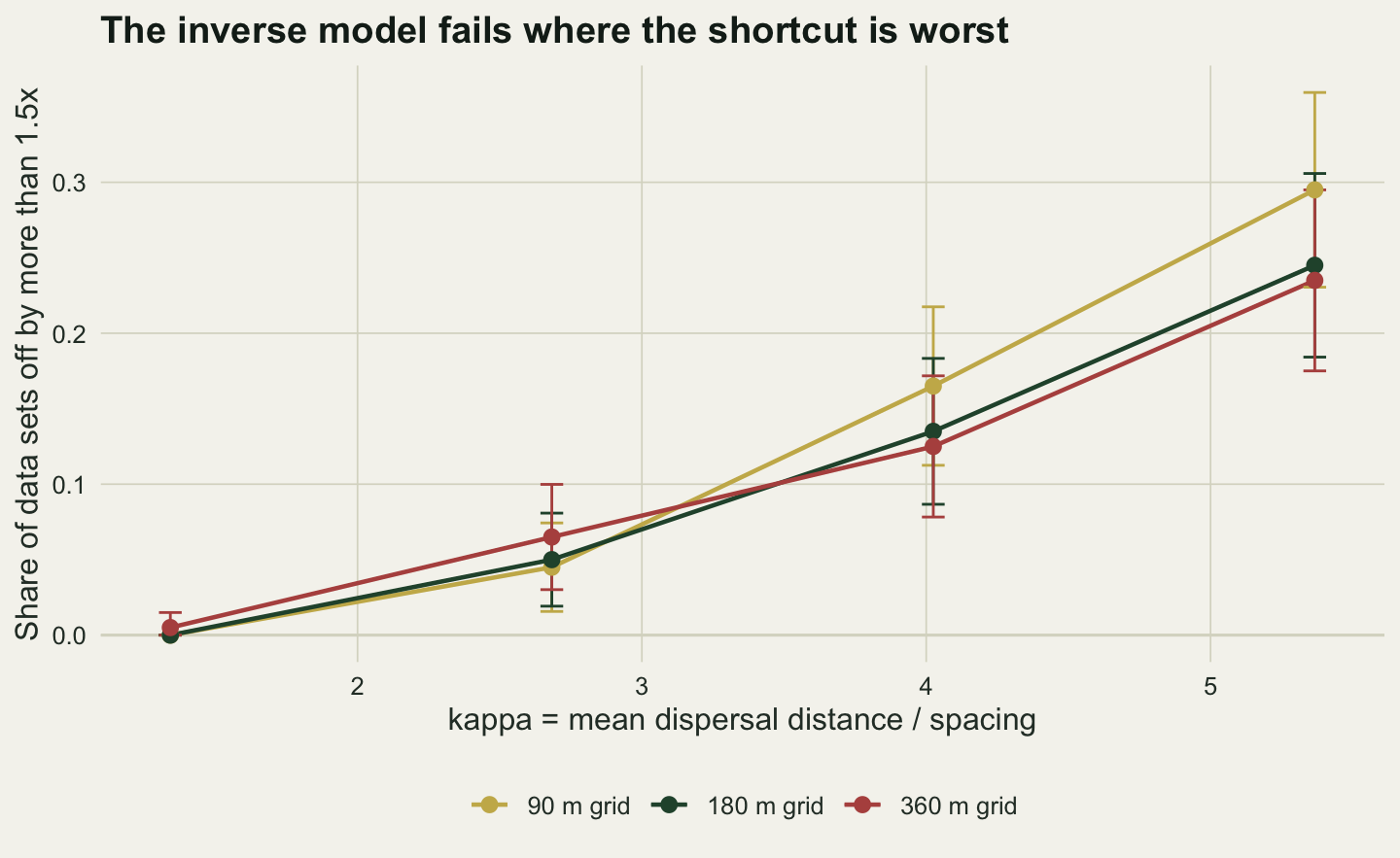
The grid side barely moves the curve. At kappa 5.4, quadrupling it from 90 to 360 m lowers the failure share by 0.060, against a combined Monte Carlo standard error of 0.044. At a fixed catch of about 3 seeds per trap, the limit is set by kappa, not by the size of the grid relative to the kernel: at the same ratio of grid side to mean distance, three, a 30 m kernel on the 90 m grid fails in 0.045 of data sets and a 60 m kernel on the 180 m grid in 0.245. A wider grid adds traps further from the centre, but at a wide kernel they sit under the same smooth rain.
The ridge in the profile likelihood
A point estimate whose median is right and which is wrong a quarter of the time is sitting on a flat likelihood. The profile negative log-likelihood of the scale, with fecundity re-profiled at each value, shows that directly, and the likelihood-ratio interval (every scale whose profile lies within qchisq(0.95, 1) / 2, about 1.92, of the minimum) is the matching summary. The figure below draws the profile for 20 fresh data sets at each of two kernels on the 180 m grid.
set.seed(3274)
log_ratio_grid <- seq(log(1 / 4), log(400 / 30), length.out = 60)
profile_df <- do.call(rbind, lapply(c(30, 60), function(mu) {
  do.call(rbind, lapply(seq_len(20), function(k) {
    td <- trap_data(20, mu, 180)
    la <- log(mu / 2) + log_ratio_grid
    la <- la[exp(la) >= a_bounds[1] & exp(la) <= a_bounds[2]]
    nll <- sapply(la, scale_nll, y = td$y, dist = td$dist)
    data.frame(ratio = exp(la) / (mu / 2), dnll = nll - min(nll), set = k,
               panel = sprintf("mean distance %d m, kappa %.1f", mu, kappa_of(20, mu)))
  }))
}))
int_rows <- sweep_tab[sweep_tab$extent == 180, c("mu", "kappa", "median", "fail",
                                                  "width", "cover")]
print(format(int_rows, digits = 3), row.names = FALSE)
mu kappa median fail width cover
15 1.34 0.994 0.000 1.39 0.950
30 2.68 0.972 0.050 1.91 0.935
45 4.02 0.970 0.135 2.86 0.935
60 5.37 1.024 0.245 7.42 0.960On the 180 m grid the median interval spans a factor of 1.4 from lower to upper limit at kappa 1.3, 1.9 at 2.7, 2.9 at 4.0 and 7.4 at 5.4, and it covers the true scale in 0.935 to 0.960 of data sets across the four kappas, against a nominal 0.95. The interval keeps its promise at every kappa, including the ones where the point estimate fails: at kappa 5.4 it says, correctly, that 100 traps pin the scale down only to within a factor of about 7. Reporting it instead of the point estimate makes the failure visible; it does not remove it.
ggplot(profile_df, aes(ratio, dnll, group = set)) +
  geom_hline(yintercept = qchisq(0.95, 1) / 2, linetype = 2, colour = te_rust,
             linewidth = 0.4) +
  geom_vline(xintercept = 1, colour = te_body, linewidth = 0.3) +
  geom_line(colour = te_forest, alpha = 0.7, linewidth = 0.5) +
  facet_wrap(~ panel) +
  scale_x_log10(breaks = c(0.25, 0.5, 1, 2, 4, 8),
                labels = c("1/4", "1/2", "1", "2", "4", "8")) +
  coord_cartesian(ylim = c(0, 8)) +
  labs(x = "Kernel scale / true scale", y = "Profile negative log-likelihood above its minimum") +
  theme_datasheet() +
  theme(strip.text = element_text(colour = te_ink, face = "bold"))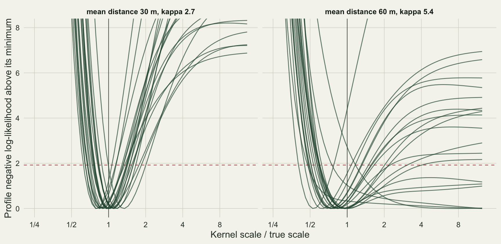
At kappa 2.7 every curve is a narrow valley around the true scale. At kappa 5.4 the left wall is still steep, because a kernel much shorter than the truth would predict relief the traps do not see, but the right side is a long shallow slope: a kernel two or four times too wide costs far less than the same factor in the short direction, and in a few data sets the minimum sits at the far end, where the kernel is so wide that the rain is flat. The asymmetry has a practical reading. At wide kappa the inverse model can rule out a short kernel; it cannot say how long the long one is.
More seeds, not a wider grid
If a wide kernel fails because each seed carries little information about the scale, more seeds should help and a wider grid should not, and the sweep has already shown the second half. The controls sit on the 180 m grid at kappa 5.4 unless stated, 200 data sets each. Three add information in different ways: fecundity known to the model instead of profiled, three and ten times the seed output per adult (which is what pooling three or ten years of catches from the same adults, or larger traps, would give), and 196 traps in a 14 x 14 grid over the same square. Two break the model’s assumptions: lognormal fecundity (sdlog 1) that the model does not know about, and Thomas-clustered adults, each at kappa 2.7 and 5.4. The last control is the other failure cause, a sparse rain: 2 adults per hectare with a 40 m kernel, a modest kappa but few seeds in each trap.
set.seed(3275)
ctrl_spec <- list(
  list(lab = "fecundity known to the model", mu = 60, known = TRUE),
  list(lab = "3x seeds per adult", mu = 60, seeds = 3 * seeds_per_adult),
  list(lab = "10x seeds per adult", mu = 60, seeds = 10 * seeds_per_adult),
  list(lab = "196 traps (14 x 14)", mu = 60, n_side = 14),
  list(lab = "unequal fecundity, unknown", mu = 30, fec_sd = 1),
  list(lab = "unequal fecundity, unknown", mu = 60, fec_sd = 1),
  list(lab = "Thomas clustered adults", mu = 30, pattern = "thomas"),
  list(lab = "Thomas clustered adults", mu = 60, pattern = "thomas"),
  list(lab = "2 adults per ha, 40 m", mu = 40, dens = 2))
ctrl_tab <- do.call(rbind, lapply(ctrl_spec, function(s) {
  r <- run_cell(n_rep_inv, if (is.null(s$dens)) 20 else s$dens, s$mu, 180,
                pattern = if (is.null(s$pattern)) "poisson" else s$pattern,
                fec_sd = if (is.null(s$fec_sd)) 0 else s$fec_sd,
                seeds = if (is.null(s$seeds)) seeds_per_adult else s$seeds,
                n_side = if (is.null(s$n_side)) 10 else s$n_side,
                known = isTRUE(s$known))
  cbind(arm = s$lab, r)
}))
ctrl_tab$fail_se <- sqrt(ctrl_tab$fail * (1 - ctrl_tab$fail) / n_rep_inv)
print(format(ctrl_tab[, c("arm", "mu", "kappa", "median", "q25", "q75", "fail",
                          "fail_se", "at_bound", "seeds_trap")], digits = 3),
      row.names = FALSE)
arm mu kappa median q25 q75 fail fail_se at_bound
fecundity known to the model 60 5.37 1.074 0.833 1.41 0.245 0.03041 0.000
3x seeds per adult 60 5.37 0.986 0.889 1.12 0.050 0.01541 0.005
10x seeds per adult 60 5.37 1.009 0.937 1.09 0.005 0.00499 0.000
196 traps (14 x 14) 60 5.37 1.009 0.857 1.15 0.085 0.01972 0.015
unequal fecundity, unknown 30 2.68 0.983 0.890 1.15 0.075 0.01862 0.015
unequal fecundity, unknown 60 5.37 0.975 0.792 1.44 0.340 0.03350 0.040
Thomas clustered adults 30 2.68 1.015 0.933 1.10 0.005 0.00499 0.000
Thomas clustered adults 60 5.37 0.996 0.900 1.16 0.060 0.01679 0.000
2 adults per ha, 40 m 40 1.13 0.986 0.856 1.24 0.130 0.02378 0.005
seeds_trap
3.002
8.971
30.074
2.971
3.051
3.015
2.968
2.970
0.298ctrl_of <- function(lab, mu) ctrl_tab[ctrl_tab$arm == lab & ctrl_tab$mu == mu, ]Knowing fecundity made no detectable difference: the failure share is 0.245 with fecundity fixed at its true value against 0.245 with it profiled, so the joint fit is not what flattens the ridge; far from the stand edge the total catch carries little information about the scale in the first place. More seeds help quickly: 0.050 of data sets fail at three times the output and 0.005 at ten times, with 9.0 and 30.1 seeds per trap. Nearly doubling the number of traps inside the same square gives 0.085. Fecundity that varies among adults, when the model assumes it equal, makes things worse: 0.340 at kappa 5.4 and 0.075 at 2.7, against 0.245 and 0.050 with equal fecundity. Clustered adults help at kappa 5.4 (0.060, and 0.005 at 2.7), because clumps of trees put back some of the relief that a wide kernel smooths away; that is a property of the stand, not something a sampling design can choose. The sparse stand fails in 0.130 of data sets at a kappa of only 1.13, with 0.30 seeds per trap. That failure has a different cause, too few seeds in total rather than too little relief per seed, but the same cure.
So the answer to how large the trap grid must be is that its size is the wrong lever. At 20 adults per hectare and about 3 seeds per trap, a grid three kernel means wide identifies the scale at kappa 2.7 and does not at kappa 5.4, and making it four times wider changes little. What moves the failure share is the number of seeds caught, through trap area, trap number or years of catches.
What to report
Compute kappa before the fieldwork, from the stand’s adult density and a prior guess of the mean dispersal distance, and print it. If it is above about one, about half the seedlings or more are given the wrong adult (0.46 at kappa 1); above about two, nearest-adult distances describe the spacing of the stand, and the wrong-parent share and the shrinkage of the mean are given by the two integrals above; there is no need to simulate them. Quote the formula’s numbers for the reader’s own stand rather than a general warning.
For an inverse model, report the profile-likelihood interval for the scale beside the point estimate, and say whether the maximum sat on the edge of the search interval. Report the grid side and the trap spacing in units of the fitted mean distance, and the mean catch per trap. With those numbers a reader can place the fit on the curves above. For a wide kernel fitted from a few seeds per trap, only the lower limit of the interval is informative; the data rule out a short kernel and say little about how long the long one is.
When kappa is large, spend the effort on seeds caught rather than on grid extent. At kappa 5.4 in this design, three times the catch brought the failure share from 0.245 to 0.050, while a grid four times wider did not bring it below 0.235.
Honest limits
The closed form needs a Poisson pattern of adults. Clustering barely moved it here, but a regular stand, where adults inhibit each other, has a narrower nearest-neighbour distribution and would need its own empty-space function in place of exp(-lambda * pi * r^2). The formula also counts seeds, or seedlings whose survival does not depend on where the other adults stand. Where mortality is higher near conspecific adults, the survivors sit farther from the nearest adult than a random seed would; a seedling that escaped every adult is usually one that travelled far from its own, so the wrong-parent share among the survivors is higher than the integral gives, not lower. The kernel is the two-dimensional exponential throughout; a fat-tailed kernel keeps the same cap on the shortcut, since the cap comes from D alone, but its wrong-parent share and the inverse model’s behaviour were not run.
The inverse model here is the most favourable version of itself: the right kernel family, every adult mapped, no adults outside the stand, Poisson counts without overdispersion, and seeds counted where they land rather than seedlings after post-dispersal mortality. Each of those departures removes information or adds a nuisance parameter, and none was simulated, so the failure shares are for a best case. Hardesty and colleagues give a field measure of how much that best case can flatter: for their tree, inverse modelling of seedling recruitment put the mean recruitment distance at 39 m against 392 m from parentage. The trap design is one design, 100 traps of 0.5 square metres at a mean of 3 seeds per trap, and the threshold of 1.5x is a choice; a stricter threshold raises every failure share and a looser one lowers them, but the ordering by kappa is what the post relies on.
Parentage is left out. With genotypes, the problem changes from fitting a scale to excluding candidate mothers, and at kappa 5.4 a seedling has on average about 23 adults within one mean dispersal distance of it (that is pi * kappa^2 / 4, from the Poisson density again), so exclusion has to be strong for parentage to beat the inverse model there. Jones and Muller-Landau compared classical and genetic methods for long-distance dispersal on the same tree, and a reader with genotypes should start there; whether a realistic exclusion rate wins at kappa 5 was not simulated for this post.
Finally, the Monte Carlo numbers carry their own error: each inverse cell is 200 data sets, so failure shares near a quarter carry standard errors of about 0.03, and differences of a few hundredths between neighbouring cells are not worth reading.
References
Nathan R, Muller-Landau HC 2000 Trends in Ecology & Evolution 15(7):278-285 (10.1016/S0169-5347(00)01874-7)
Hardesty BD, Hubbell SP, Bermingham E 2006 Ecology Letters 9(5):516-525 (10.1111/j.1461-0248.2006.00897.x)
Ribbens E, Silander JA, Pacala SW 1994 Ecology 75(6):1794-1806 (10.2307/1939638)
Clark JS, Silman M, Kern R, Macklin E, HilleRisLambers J 1999 Ecology 80(5):1475-1494 (10.1890/0012-9658(1999)080[1475:SDNAFP]2.0.CO;2)
Jones FA, Muller-Landau HC 2008 Journal of Ecology 96(4):642-652 (10.1111/j.1365-2745.2008.01400.x)