library(ggplot2)

te_paper  <- "#f5f4ee"
te_ink    <- "#16241d"
te_body   <- "#2c3a31"
te_forest <- "#275139"
te_rust   <- "#b5534e"
te_gold   <- "#c9b458"
te_line   <- "#dad9ca"

theme_datasheet <- function() {
  theme_minimal(base_size = 12) +
    theme(plot.background  = element_rect(fill = te_paper, colour = NA),
          panel.background = element_rect(fill = te_paper, colour = NA),
          panel.grid.major = element_line(colour = te_line, linewidth = 0.3),
          panel.grid.minor = element_blank(),
          text             = element_text(colour = te_body),
          plot.title       = element_text(colour = te_ink, face = "bold"),
          axis.text        = element_text(colour = te_body))
}

# wrap a coordinate difference onto the torus: the shortest signed offset
wrap <- function(d) d - round(d)Plotless density estimation from distances
R
spatial
point patterns
sampling
ecology tutorial
Convert point-to-tree distances into density in base R: why the nearest-tree estimator fails on clustered woodland, and how far T-square sampling repairs it.
Corrected 30 September 2026: the post said an index near one half means the naive density is unbiased and that a high index means an order-of-magnitude error; it now says an index near one half gives no evidence against randomness, which does not prove the estimate unbiased, and ties the order-of-magnitude error to the clustered pattern simulated here.
You need stems per hectare from a steep beech stand with a hazel understorey too thick for a tape to cross in a straight line. Plotless methods offer a way out of laying quadrats there: walk to a random point, measure the distance to the nearest tree, repeat about a hundred times, and turn the distances into a density with one line of arithmetic.
The arithmetic is exact, and it is exact under exactly one condition: that the trees are laid out completely at random. Real vegetation almost never is.
There is a sharper way to say that. The Clark-Evans index and the plotless density estimator are the same relation between mean distance and intensity, solved for opposite unknowns. Clark-Evans takes the density as known and asks whether the pattern is random; the plotless estimator takes the pattern as random and asks what the density is. The assumption one tests is the assumption the other needs, and no set of distances supplies both.
One equation, two unknowns
Under complete spatial randomness with intensity lambda, the disc of radius r around any fixed location is empty with probability exp(-lambda * pi * r^2). The squared distance to the nearest tree is exponential with mean 1 / (pi * lambda), and the distance itself is Rayleigh with mean 1 / (2 * sqrt(lambda)).
Read that mean from right to left and you have Clark-Evans: divide the observed mean nearest-neighbour distance by 1 / (2 * sqrt(lambda)) and see whether the ratio is one. Read it from left to right and you have the plotless estimator: set the observed mean equal to the expected one and solve.
\[ \hat\lambda \;=\; \frac{1}{4\,\bar r^{\,2}} \qquad\text{or, from the squared distances,}\qquad \hat\lambda \;=\; \frac{m-1}{\pi \sum_{i=1}^{m} r_i^{2}} . \]
The second form is the one to survey with: the squared distances are exponential, so m - 1 rather than m makes the estimator unbiased. The first is biased upward by Jensen’s inequality, but it is built on a mean distance exactly as Clark-Evans is, so it is the form the next section uses.
Three woodlands at the same density
The window is the unit square, so a count of 400 trees is an intensity of 400 per unit area and the truth is known by construction. The three patterns differ only in arrangement: one random, one made of twenty offspring clouds around random parents, one thinned by a minimum spacing rule.
n_trees <- 400
lambda_true <- n_trees          # unit square: count and intensity coincide

gen_csr <- function(n) data.frame(x = runif(n), y = runif(n))

gen_clust <- function(n, n_parent = 20, sd_off = 0.02) {
  px <- runif(n_parent); py <- runif(n_parent)
  k  <- sample(n_parent, n, replace = TRUE)
  data.frame(x = (px[k] + rnorm(n, 0, sd_off)) %% 1,
             y = (py[k] + rnorm(n, 0, sd_off)) %% 1)
}

gen_reg <- function(n, d_min = 0.038) {
  ax <- numeric(n); ay <- numeric(n); got <- 0
  while (got < n) {
    qx <- runif(1); qy <- runif(1)
    if (got == 0) {
      got <- 1; ax[1] <- qx; ay[1] <- qy
    } else if (min(wrap(ax[1:got] - qx)^2 + wrap(ay[1:got] - qy)^2) >= d_min^2) {
      got <- got + 1; ax[got] <- qx; ay[got] <- qy
    }
  }
  data.frame(x = ax, y = ay)
}

# distance from every tree to its nearest neighbouring tree
nn_tree <- function(p) sapply(seq_len(nrow(p)), function(i) {
  d2 <- wrap(p$x - p$x[i])^2 + wrap(p$y - p$y[i])^2
  sqrt(min(d2[-i]))
})

set.seed(20260813)
patterns <- list(random    = gen_csr(n_trees),
                 clustered = gen_clust(n_trees),
                 regular   = gen_reg(n_trees))
nn_all <- lapply(patterns, nn_tree)
sapply(patterns, nrow)
random clustered regular
400 400 400 At each sample point the survey records the distance to the nearest tree, a second distance onward from that tree into the half plane beyond it, and the nearest tree in each of four quadrants.
The edge problem has to be settled first. A sample point near the boundary may have its true nearest tree just outside the window, so the recorded distance is too long and the density too low. I wrap the square onto a torus, left edge glued to right and top to bottom, so any bias below belongs to the estimator rather than to the window. The field equivalent is an inner buffer costing 36 per cent of the plot at one tenth of the side, and it has to be wider than the longest walk you expect.
survey <- function(trees, m) {
  ox <- runif(m); oy <- runif(m)
  tx <- trees$x;  ty <- trees$y
  quadrants <- list(c(1, 1), c(1, -1), c(-1, 1), c(-1, -1))
  out <- t(sapply(seq_len(m), function(i) {
    dx <- wrap(tx - ox[i]); dy <- wrap(ty - oy[i])
    d2 <- dx^2 + dy^2
    j  <- which.min(d2)                       # the nearest tree
    # T-square: from that tree, look only into the half plane beyond it
    qx <- wrap(tx - tx[j]); qy <- wrap(ty - ty[j])
    beyond <- (qx * dx[j] + qy * dy[j]) > 0
    quad <- sapply(quadrants, function(s) {
      sel <- sign(dx) == s[1] & sign(dy) == s[2]
      if (any(sel)) sqrt(min(d2[sel])) else NA_real_
    })
    c(sqrt(d2[j]), sqrt(min(qx[beyond]^2 + qy[beyond]^2)), quad, j)
  }))
  data.frame(ox = ox, oy = oy, x = out[, 1], z = out[, 2],
             q1 = out[, 3], q2 = out[, 4], q3 = out[, 5], q4 = out[, 6],
             tree = out[, 7])          # which tree, so shared ones can be counted
}

lam_point <- function(s) (nrow(s) - 1) / (pi * sum(s$x^2))   # Pollard form
lam_ray   <- function(s) 1 / (4 * mean(s$x)^2)               # Rayleigh mean form
A picture first. Each panel holds the same number of trees, and each open circle is the empty disc around one of fifteen random sample points.
set.seed(11)
demo <- lapply(patterns, function(p) survey(p, 15))

circle_path <- function(s) {
  th <- seq(0, 2 * pi, length.out = 80)
  do.call(rbind, lapply(seq_len(nrow(s)), function(i)
    data.frame(id = i, x = s$ox[i] + s$x[i] * cos(th),
               y = s$oy[i] + s$x[i] * sin(th))))
}

tree_df <- do.call(rbind, lapply(names(patterns), function(nm)
  data.frame(pattern = nm, patterns[[nm]])))
disc_df <- do.call(rbind, lapply(names(demo), function(nm)
  data.frame(pattern = nm, circle_path(demo[[nm]]))))
tree_df$pattern <- factor(tree_df$pattern, levels = names(patterns))
disc_df$pattern <- factor(disc_df$pattern, levels = names(patterns))

ggplot(tree_df, aes(x, y)) +
  geom_point(colour = te_ink, size = 0.55, alpha = 0.8) +
  geom_path(data = disc_df, aes(group = id), colour = te_rust, linewidth = 0.5) +
  facet_wrap(~ pattern) +
  coord_fixed(xlim = c(0, 1), ylim = c(0, 1)) +
  labs(x = NULL, y = NULL, title = "Same density, three arrangements") +
  theme_datasheet() +
  theme(axis.text = element_blank())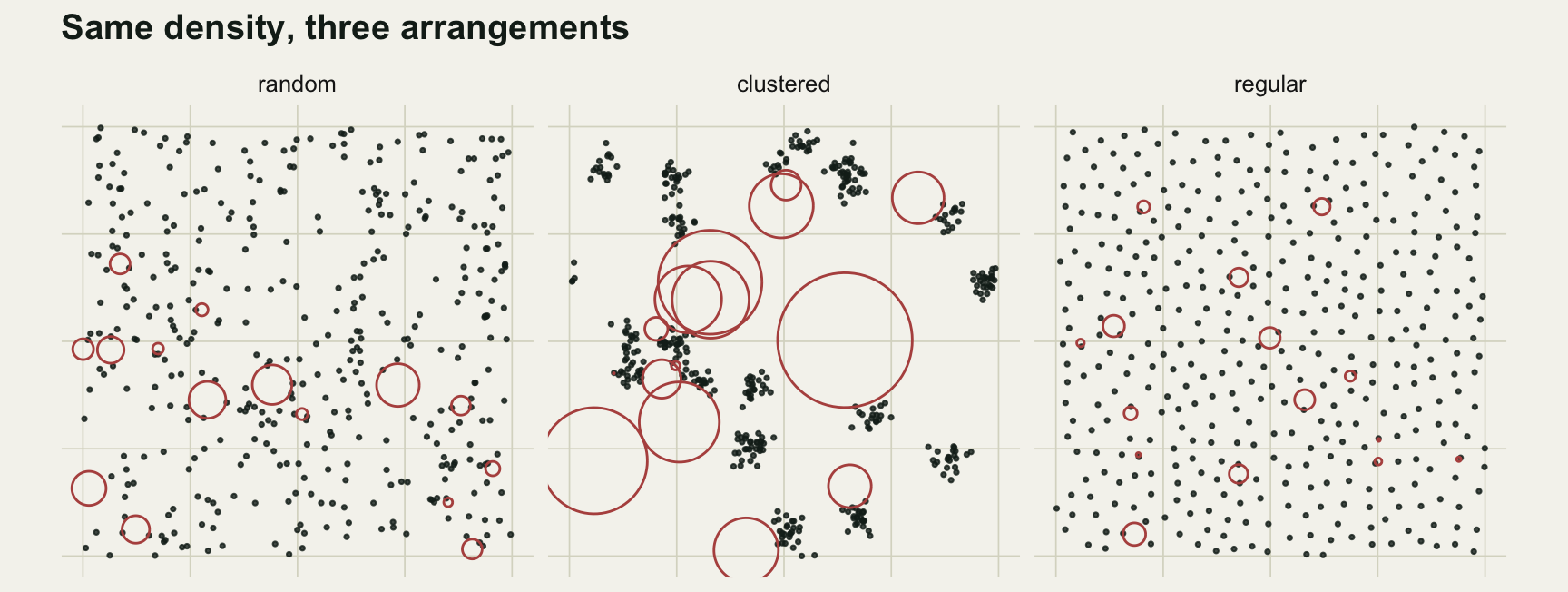
The naive estimate, and its mirror image
Run a large survey on each pattern and compare two averages that coincide under randomness: sample point to nearest tree, and tree to nearest tree. Both have expectation 1 / (2 * sqrt(lambda)), so one formula serves for both.
set.seed(19)
big <- lapply(patterns, function(p) survey(p, 2000))

crux <- data.frame(
  pattern      = names(patterns),
  point_tree   = round(sapply(big, function(s) mean(s$x)), 4),
  tree_tree    = round(sapply(nn_all, mean), 4),
  lam_from_pt  = round(sapply(big, lam_ray)),
  lam_from_nn  = round(sapply(nn_all, function(d) 1 / (4 * mean(d)^2))),
  clark_evans  = round(sapply(nn_all, function(d) mean(d) * 2 * sqrt(lambda_true)), 3))
print(crux, row.names = FALSE)
pattern point_tree tree_tree lam_from_pt lam_from_nn clark_evans
random 0.0255 0.0244 385 418 0.978
clustered 0.0774 0.0089 42 3127 0.358
regular 0.0196 0.0417 654 144 1.667On the random pattern the two averages are within 4.5 per cent of each other, and the two formulas land at 385 and 418 against a truth of 400. That gap is the luck of one realisation: this random pattern has a Clark-Evans index of 0.98 rather than exactly one.
On the clustered pattern they come apart completely. The mean walk from a sample point to a tree is 0.0774, about 3.0 times the random value, because most of the ground is gap and most sample points land in one; the mean distance from a tree to its neighbour is 0.0089, shorter by a factor of 2.7, because every tree is inside a clump. The same equation therefore reports 42 trees per unit area from the sample points and 3127 from the trees, out by about 10 downward and 8 upward against a truth of 400. Both come from one realisation, and clustered patterns swing between realisations far more than random ones; the replicated table below is the one to quote.
The regular pattern splits them the same way and more mildly, 654 from the sample points against 144 from the trees, because inhibition leaves no large voids for a sample point to land in while pushing the trees themselves apart.
The last column, Clark-Evans on the same tree-to-tree distances with lambda set to its true value, is that arithmetic run backwards. Knowing the index requires knowing the density; getting the density from distances alone requires assuming the index is one.
Quarters and T-squares
Two field methods try to break out of this. The point-centred quarter method splits the view at each sample point into four quadrants and measures the nearest tree in each, so a hundred points yield four hundred distances whenever no quadrant is empty. The T-square method measures a second distance of a different kind: from the nearest tree it looks only into the half plane beyond a line drawn through that tree at right angles to your approach.
The quarter method still measures outward from the sample point, so all four distances inherit the same inflation in a gap: it buys precision, not protection. A T-square distance is a tree-to-tree distance, and those move the opposite way under clustering. Write x for the point-to-tree distance and z for the T-square one. The half plane halves the search area, so under randomness z^2 is exponential with twice the mean of x^2, giving E[z] = sqrt(2) * E[x] and a product of expectations of 1 / (2 * sqrt(2) * lambda). Solve for lambda and you have the Byth and Ripley compound estimator, in which x inflated by clustering and z deflated by it cancel part of the error.
\[ \hat\lambda_{T} \;=\; \frac{m^{2}}{2\sqrt{2}\,\left(\sum_i x_i\right)\left(\sum_i z_i\right)} \]
The trial: two hundred independent surveys per arrangement, a fresh pattern and fresh sample points each time, a hundred sample points per survey. The row labelled double is the point-to-tree estimator walking to two hundred points instead of one hundred, so it spends the same number of measurements as the T-square survey. The point-to-tree and quarter rows are both written in the squared-distance form, so the difference between those two is a difference of method rather than of formula; the T-square row keeps the Byth-Ripley form, which is the form that estimator comes in. It is also why these numbers sit away from the table above, which used the mean-distance form on one realisation.
# a quadrant is a quarter of the plane, so E[q^2] = 4 / (pi * lambda)
lam_quarter <- function(s) {
  q <- as.matrix(s[, c("q1", "q2", "q3", "q4")])
  q <- q[!is.na(q)]
  4 * (length(q) - 1) / (pi * sum(q^2))
}

lam_tsquare <- function(s)
  nrow(s)^2 / (2 * sqrt(2) * sum(s$x) * sum(s$z))

t_index <- function(s) mean(s$x^2 / (s$x^2 + s$z^2 / 2))

gens <- list(random    = function() gen_csr(n_trees),
             clustered = function() gen_clust(n_trees),
             regular   = function() gen_reg(n_trees))

set.seed(2026)
m_pts <- 100
reps <- do.call(rbind, lapply(names(gens), function(nm) {
  out <- t(replicate(200, {
    p <- gens[[nm]](); s <- survey(p, 2 * m_pts); h <- s[1:m_pts, ]
    c(nearest = lam_point(h), quarter = lam_quarter(h), tsquare = lam_tsquare(h),
      double = lam_point(s), t = t_index(h))
  }))
  data.frame(pattern = nm, as.data.frame(out))
}))

stat_row <- function(v) data.frame(mean = round(mean(v)), sd = round(sd(v), 1),
                                  rmse = round(sqrt(mean((v - lambda_true)^2))))
stats <- do.call(rbind, lapply(names(gens), function(nm)
  do.call(rbind, lapply(c("nearest", "quarter", "tsquare", "double"), function(e)
    cbind(data.frame(pattern = nm, estimator = e),
          stat_row(reps[[e]][reps$pattern == nm]))))))
val <- function(pat, est, what)
  stats[[what]][stats$pattern == pat & stats$estimator == est]
print(stats, row.names = FALSE)
pattern estimator mean sd rmse
random nearest 397 47.3 47
random quarter 399 25.2 25
random tsquare 398 30.5 31
random double 400 32.1 32
clustered nearest 38 8.5 362
clustered quarter 40 7.9 360
clustered tsquare 262 38.9 143
clustered double 38 8.1 362
regular nearest 696 52.7 301
regular quarter 674 15.7 274
regular tsquare 396 18.1 19
regular double 699 36.1 301rand <- reps[reps$pattern == "random", ]
set.seed(88)
paired <- replicate(20000, {
i <- sample(nrow(rand), replace = TRUE)
sd(rand$tsquare[i]) - sd(rand$double[i])
})
naive_span <- round(quantile(rand$nearest, c(0.05, 0.95)))
round(c(gap = sd(rand$tsquare) - sd(rand$double), se_paired = sd(paired),
se_single = sd(rand$tsquare) / sqrt(2 * nrow(rand) - 2)), 2) gap se_paired se_single
-1.62 2.04 1.53 The random pattern is the calibration, and all four rows sit within a few per cent of the truth there. Four distances at a hundred sample points gives the quarter method a spread of 25.2 against 47.3 for one distance at the same points, a factor of 1.88, close to the halving that four times the data should buy.
The pair worth staring at is the T-square survey at 30.5 and the doubled point-to-tree survey at 32.1, which spend the same number of measurements. They differ by 1.6, and the yardstick is not the 1.5 standard error of a single spread: the two columns share their first hundred sample points, so the difference has to be resampled in pairs, which gives about 2.0. A second distance at a sample point is worth about as much as a first distance at a new one, and the received warning that resistance has to be paid for in variance did not show up here.
On the clustered pattern the naive estimator collapses to 38, or 9.5 per cent of the truth, and the quarter method reports 40. Four distances per point have left the bias where it was and cut the spread by a factor of only 1.08, against the 1.88 they bought on random ground. All four are measured outward from a sample point that fell in a gap, so all four are inflated together: averaging them cancels the noise between them and none of the error they share. Precision is not protection, and on clumped ground the quarter method delivers little of either.
The T-square estimator reports 262, still low by 34.5 per cent: a long way from correct and a long way better, with a root mean squared error of 143 against 362. On the regular pattern the cancellation does nearly all of the work: the naive estimator overshoots to 696 and the quarter method to 674, the same failure twice over now that both are read off the same formula, while the T-square estimator returns 396 against a truth of 400, with the smallest root mean squared error in the table.
long <- do.call(rbind, lapply(c("nearest", "quarter", "tsquare"), function(e)
  data.frame(pattern = reps$pattern, estimator = e,
             ratio = reps[[e]] / lambda_true)))
long$estimator <- factor(long$estimator, levels = c("tsquare", "quarter", "nearest"),
                         labels = c("T-square", "point-centred quarter", "nearest tree"))
long$pattern <- factor(long$pattern, levels = names(gens))

ggplot(long, aes(x = ratio, y = estimator, colour = estimator)) +
  geom_vline(xintercept = 1, linetype = "dashed", colour = te_body) +
  geom_boxplot(outlier.size = 0.6, linewidth = 0.5) +
  scale_x_log10(breaks = c(0.1, 0.25, 0.5, 1, 2)) +
  scale_colour_manual(values = c(te_forest, te_gold, te_rust)) +
  facet_wrap(~ pattern, ncol = 1) +
  labs(x = "estimated density / true density", y = NULL,
       title = "Where each estimator lands when the trees are not random") +
  theme_datasheet() +
  theme(legend.position = "none")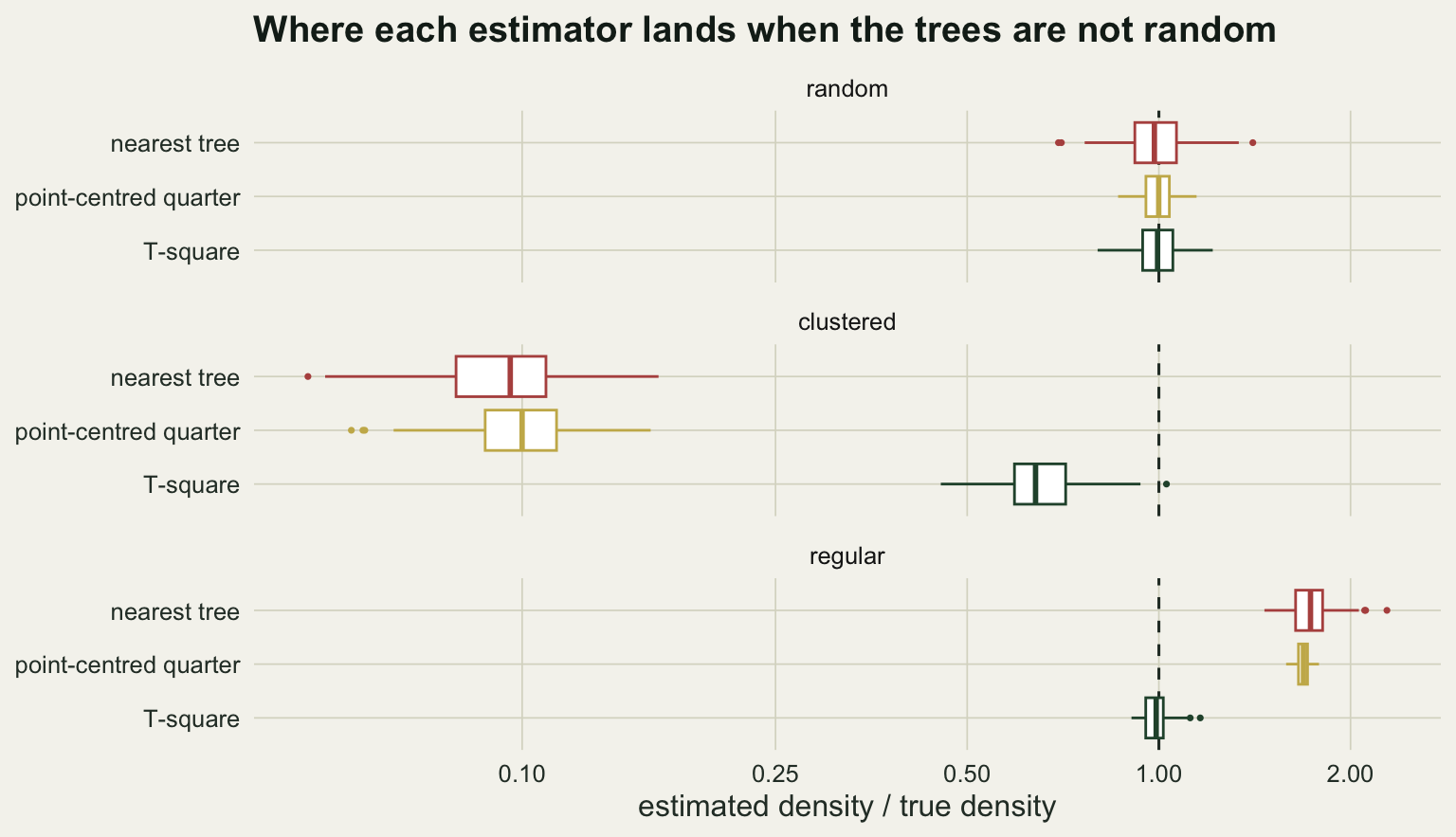
A randomness test from the same distances
The pair of distances at each sample point carries one more thing. Under complete spatial randomness x^2 and z^2 / 2 are independent exponentials with the same mean, so their ratio
\[ t_i \;=\; \frac{x_i^{2}}{x_i^{2} + z_i^{2}/2} \]
is uniform on the unit interval. Average the t_i over m sample points and the mean is one half whatever the density is. Clumping makes x long and z short and pushes the average above a half; inhibition pushes it below. This is the T-square index of randomness, and it tests exactly the assumption the density estimator has to make.
The textbook variance of that average is 1 / (12 * m), and it holds only if the m sample points carry independent information. At one sample point per four stems they do not: points that land near each other walk to the same tree. Rather than assume the null, simulate it, and count the sharing on the way past.
set.seed(404)
shared <- replicate(200, length(unique(survey(gen_csr(n_trees), m_pts)$tree)))

m_grid <- c(25, 100, 200)
null_t <- lapply(m_grid, function(m)
  replicate(2000, t_index(survey(gen_csr(n_trees), m))))

null_tab <- data.frame(
  m          = m_grid,
  sd_null    = round(sapply(null_t, sd), 4),
  sd_formula = round(1 / sqrt(12 * m_grid), 4),
  size_pct   = round(100 * mapply(function(v, m)
                     mean(abs(v - 0.5) > 1.96 / sqrt(12 * m)), null_t, m_grid), 1))
print(null_tab, row.names = FALSE)
m sd_null sd_formula size_pct
25 0.0584 0.0577 4.9
100 0.0306 0.0289 6.6
200 0.0235 0.0204 8.7t_lim <- quantile(null_t[[2]], c(0.025, 0.975)) # simulated limits at m = 100Twenty-five points on four hundred trees is sparse enough for the formula to be about right: the simulated spread is 0.0584 against the assumed 0.0577. At the hundred this post surveys with, only 86.5 distinct trees on average are anybody’s nearest tree, the simulated spread is 0.0306, and limits set at 1.96 / sqrt(12 * m) reject 6.6 per cent of random surveys instead of five. At two hundred points, 8.7 per cent. Each of those rates rests on two thousand simulated surveys and carries about half a percentage point of noise, so read the trend rather than the digits: the more densely you sample a stand of a given size, the worse the formula gets, which is why the figure uses the simulated limits.
idx <- data.frame(pattern = factor(reps$pattern, levels = names(gens)), t = reps$t)

ggplot(idx, aes(x = t, colour = pattern)) +
  geom_vline(xintercept = 0.5, colour = te_body, linewidth = 0.5) +
  geom_vline(xintercept = t_lim, linetype = "dashed",
             colour = te_body, linewidth = 0.4) +
  geom_density(linewidth = 0.9) +
  scale_colour_manual(values = c(te_ink, te_rust, te_gold)) +
  labs(x = "T-square index t", y = "density", colour = NULL,
       title = "The distances test the assumption they depend on") +
  theme_datasheet() +
  theme(legend.position = "bottom")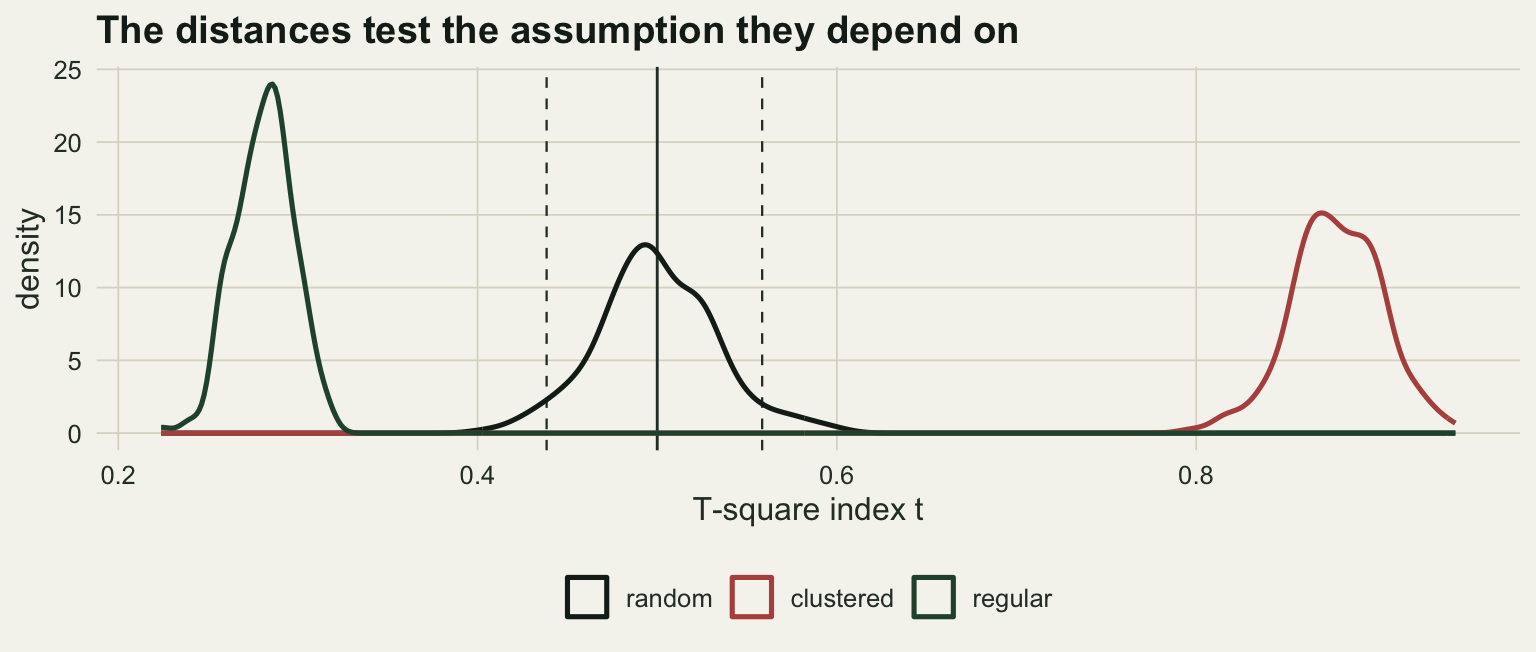
mean_t  <- tapply(reps$t, reps$pattern, mean)[names(gens)]
idx_tab <- data.frame(pattern = names(gens),
                      mean_t  = round(mean_t, 3),
                      z_score = round((mean_t - 0.5) / sd(null_t[[2]]), 1))
print(idx_tab, row.names = FALSE)
pattern mean_t z_score
random 0.500 0.0
clustered 0.878 12.4
regular 0.281 -7.2r_t <- reps$t[reps$pattern == "random"]
flagged <- c(simulated = sum(r_t < t_lim[1] | r_t > t_lim[2]),
textbook = sum(abs(r_t - 0.5) > 1.96 / sqrt(12 * m_pts)),
fair_top = qbinom(0.975, 200, 0.05)) # top of the central 95 per cent range for a true 5 per cent rate
flaggedsimulated textbook fair_top
16 20 16 The random pattern averages 0.500 with a z score of 0.0, dead on the null, but an average is not a survey. Of the 200 random surveys here, 16 fall outside the simulated limits and 20 outside the textbook ones. A true five per cent rate gives ten on average, and the top of its central 95 per cent range is 16, so the first count is within what the simulated limits allow. Two hundred surveys pin a tail rate down far too loosely to read either count as a result: the null table above, not this line, is the evidence about the textbook limits. The clustered pattern gives 0.878 and a z score of 12; the regular one 0.281 and minus 7. Both departures are unmistakable, out of the same hundred pairs of measurements that produced the density estimate.
That is the practical resolution of the circularity. One survey still cannot give both an unbiased density and a randomness verdict: the index says the assumption is broken without saying how wrong the estimate is. What it gives is a warning label. Near a half the index gives no evidence against randomness, which is not proof that the naive number is unbiased, and even on truly random ground a hundred sample points leave nine surveys in ten anywhere between 329 and 475 against a truth of 400. At 0.88 the pattern here was clumped enough for the naive estimate to be out by an order of magnitude, and you should be counting stems in plots or at least reporting the T-square estimate and saying why.
Honest limits
Every distance here was measured on a perfect census. In a hazel understorey no tree is certain to be detected or correctly identified: a stem hidden behind another is not the one you record, and the one you do record is farther away, which pushes the estimate down in the same direction as clustering. Misidentification does the same to a single-species density. The T-square index flags neither, because a pattern thinned by imperfect detection is still close to random.
The clustered pattern uses one clustering strength: twenty parents and an offspring spread of 0.02 in a unit square. The bias scales with that spread, so there is nothing special about the multipliers above. Weaker clumping gives a smaller bias in the same direction, dense thickets in an open matrix a larger one. Real vegetation is clustered at several scales at once, which this two-scale simulation does not reproduce.
The larger problem is one the simulation cannot show, since it always samples correctly. A crew that walks a path and stops “at random” every fifty paces is not sampling at random. Paths follow ridges, edges and gaps, and stopping points along them are correlated with whatever also sets tree density. That breaks the method more thoroughly than clustering does, and in an unknown direction, where the clustering bias at least has a sign. Randomise the sample points on a map before going out.
Finally, the torus. Wrapping the window removed the edge effect so that the biases above belong to the estimators alone, but a field survey still has to handle it: an inner buffer costs sampled area, and no correction at all leaves the boundary distances long and the density low, adding to the clustering bias rather than offsetting it.
References
Cottam G, Curtis JT 1956 Ecology 37(3):451-460 (10.2307/1930167)
Pollard JH 1971 Biometrics 27(4):991-1002 (10.2307/2528833)
Diggle PJ 1975 Biometrika 62(1):39-48 (10.1093/biomet/62.1.39)
Byth K, Ripley BD 1980 Biometrics 36(2):279-284 (10.2307/2529979)
Byth K 1982 Biometrics 38(1):127-135 (10.2307/2530295)
Engeman RM, Sugihara RT, Pank LF, Dusenberry WE 1994 Ecology 75(6):1769-1779 (10.2307/1939636)