kd_2dt <- function(r, a, p) (2 * p * r / a^2) * (1 + r^2 / a^2)^(-(p + 1))
S_2dt  <- function(R, a, p) (1 + R^2 / a^2)^(-p)
m_2dt  <- function(a, p) if (p > 0.5) p * a * (sqrt(pi) / 2) * gamma(p - 0.5) / gamma(p + 1) else Inf
r2dt   <- function(N, a, p) a * sqrt((1 - runif(N))^(-1 / p) - 1)   # sampler
fit_2dt <- function(r) {
  nll <- function(v) { d <- kd_2dt(r, exp(v[1]), exp(v[2])); -sum(log(pmax(d, 1e-300))) }
  o <- tryCatch(optim(c(log(median(r)), 0), nll, method = "BFGS"),
                error = function(e) optim(c(log(median(r)), 0), nll, method = "Nelder-Mead"))
list(a = exp(o$par[1]), p = exp(o$par[2])) }Checking a dispersal kernel
R
dispersal
seed dispersal
model checking
ecology tutorial
Three checks for a fitted seed dispersal kernel in R: how far the tail rests on a few seeds, whether the trap window truncates it, and if the family matters.
Corrected 7 October 2026: Check two treated its fit of the distance density as a fit to trap counts; that density describes a distance recorded for every seed, which is what the simulation produces, while counts from equal-area traps need the per-area density, and the text now says so, as the post on fitting dispersal kernels does.
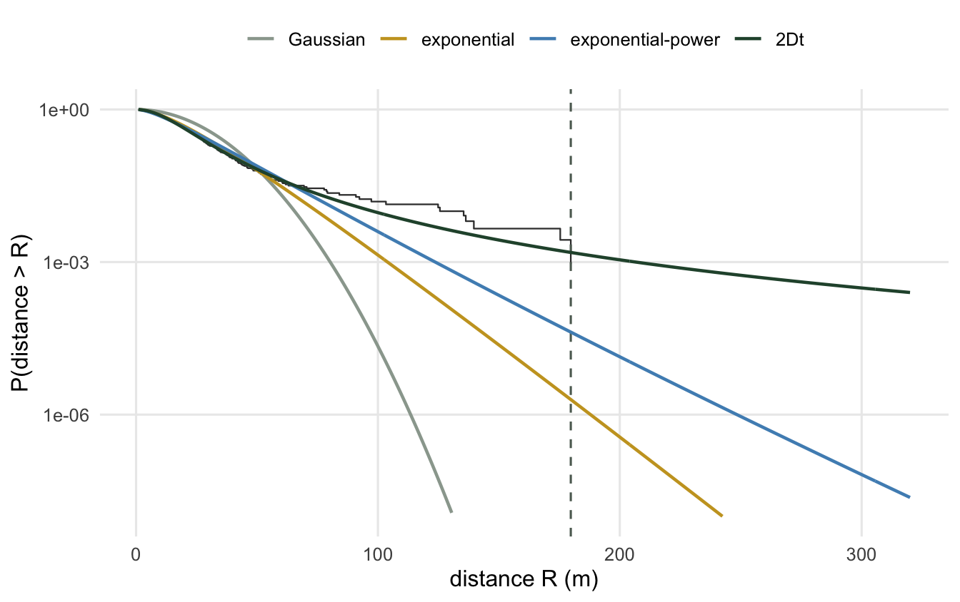
Corrected 1 October 2026: the caption of the family-comparison figure said the fitted kernels track each other within the data and diverge only past the farthest seed; they already part by orders of magnitude in the thin tail inside the data, and the caption now says so.
Corrected 30 September 2026: Check 1 read the jump in the tail exponent after trimming the farthest seeds as proof that the data had not pinned the tail down; most of that jump comes from fitting the trimmed, truncated sample without a truncation term, and the post now refits it with one and shows that the exponent holds.
Corrected 27 September 2026: the trap-window figure said the 60 m window was shaded, and its histogram used bins about 60 m wide; the shading marks the region beyond the window, which the caption now says, and the histogram now uses 5 m bins on the same density scale as the fitted curves.
The three earlier tutorials in this cluster each carried a warning: the ring geometry doubles the scale if you ignore it, the tail family sets long-distance dispersal by fiat, and the mean averages over a tail the data never saw. This one turns those warnings into checks you can run on any fitted kernel. Each targets a specific way a dispersal fit misleads, and each is a few lines of R.
Check 1: how much does the tail rest on a few seeds?
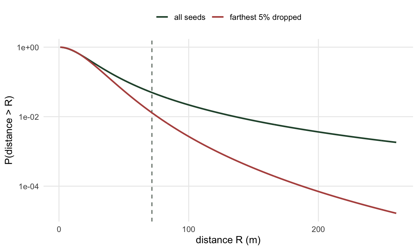
The tail exponent is estimated from the seeds that reached the tail, which are exactly the seeds you have fewest of. A quick way to feel how load-bearing they are: drop the farthest few per cent and refit. If the tail exponent barely moves, it is supported; if it jumps, it was resting on a handful of points, provided the refit allows for the cut it has just made.
set.seed(505)
r <- r2dt(500, a = 25, p = 1.3)
f_full <- fit_2dt(r)
keep <- r <= quantile(r, 0.95)          # drop the farthest 5%
f_trim <- fit_2dt(r[keep])
n_drop <- sum(!keep)
# the trimmed sample is truncated at the cut, so refit it with the Check 2 truncation term too
D_cut <- max(r[keep])
nll_cut <- function(v) { a <- exp(v[1]); p <- exp(v[2])
  -sum(log(pmax(kd_2dt(r[keep], a, p), 1e-300))) + sum(keep) * log(1 - S_2dt(D_cut, a, p)) }
p_trim_cut <- exp(optim(c(log(median(r[keep])), 0), nll_cut, method = "BFGS")$par[2])
Dropping the 25 farthest seeds (five per cent of the sample) moves the tail exponent from 1.33 to 2.83: from a heavy power-law tail to one more than twice as steep. The mean of the fitted kernel falls from 27.5 m to 23.0 m, while the median hardly stirs (20.4 m to 19.5 m). Most of that jump, though, comes from the trimming rather than from the tail: cutting the sample at a distance truncates it, and a fit that ignores the cut forces a thin tail, the failure Check 2 measures. Refit the trimmed seeds with a truncation term at the cut, as in Check 2, and the exponent comes back to 1.30. So run the check with the cut in the likelihood: only a change that survives that correction says the tail rests on a few seeds, and here the exponent holds.
Check 2: does the trap window cut off the tail?
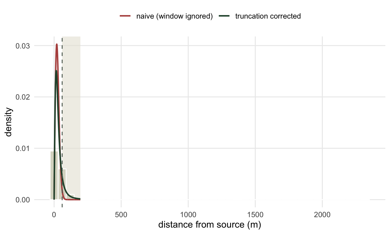
Seed traps reach only so far. Any seed that lands past the farthest trap is never counted, so the data are truncated at the window edge, and a fit that ignores this treats the truncated sample as if it were the whole kernel. Simulate a seed rain, keep only what falls within a 60 m window, and fit two ways: ignoring the truncation, and with the truncation built into the likelihood. As in the post on fitting dispersal kernels, the simulation records a distance for every seed that lands inside the window; counts from equal-area traps would need the per-area density instead, and their window cuts off the tail in the same way.
set.seed(606)
r <- r2dt(800, a = 28, p = 1.2); Dmax <- 60
obs <- r[r <= Dmax]                     # only seeds within the trap window
true_mean <- m_2dt(28, 1.2)
frac_beyond <- mean(r > Dmax); n_beyond <- sum(r > Dmax)

nll_naive <- function(v) -sum(log(pmax(kd_2dt(obs, exp(v[1]), exp(v[2])), 1e-300)))
fn <- optim(c(log(median(obs)), 0), nll_naive, method = "BFGS")
mean_naive <- m_2dt(exp(fn$par[1]), exp(fn$par[2]))

# truncated likelihood: divide the density by the probability of landing inside the window
nll_trunc <- function(v) { a <- exp(v[1]); p <- exp(v[2])
  -sum(log(pmax(kd_2dt(obs, a, p), 1e-300))) + length(obs) * log(1 - S_2dt(Dmax, a, p)) }
ft <- optim(c(log(median(obs)), 0), nll_trunc, method = "BFGS")
a_tr <- exp(ft$par[1]); p_tr <- exp(ft$par[2]); mean_trunc <- m_2dt(a_tr, p_tr)
Of the 800 seeds, 125 (15.6 per cent) landed beyond the 60 m window and never entered the data. The naive fit, treating the truncated sample as complete, reports a mean of 25.1 m against the true 35.1 m, a factor of 1.40 too low. It hits that low number by forcing an implausibly thin tail to fit inside the window. Adding a single truncation term to the likelihood, dividing the density by the probability 1 - S(D_{max}) of landing inside the window, recovers a mean of 38.4 m, back in the right range. The check is to know your window and put it in the model: a fit that never mentions the farthest distance sampled is underestimating dispersal, and the size of the miss grows with how fat the true tail is.
Check 3: does the answer survive the family?
The final check fits several kernel families to the same data and asks which conclusions hold across all of them. The ones that hold are properties of the data; the ones that swing are choices you made when you picked a family.
kd_gauss <- function(r, a) (2 * r / a^2) * exp(-(r / a)^2)
kd_exp   <- function(r, a) (r / a^2) * exp(-r / a)
kd_ep    <- function(r, a, c) (c * r / (a^2 * gamma(2 / c))) * exp(-(r / a)^c)
S_gauss  <- function(R, a) exp(-(R / a)^2); S_exp <- function(R, a) exp(-R / a) * (1 + R / a)
S_ep     <- function(R, a, c) pgamma((R / a)^c, shape = 2 / c, lower.tail = FALSE)

set.seed(707)
r <- r2dt(550, a = 24, p = 1.6)
fit1 <- function(nll, lo, hi) exp(optimize(nll, c(lo, hi))$minimum)
ag <- fit1(function(la) -sum(log(kd_gauss(r, exp(la)))), -5, 12)
ae <- fit1(function(la) -sum(log(kd_exp(r, exp(la)))), -5, 12)
op <- optim(c(log(median(r)), 0), function(v) -sum(log(pmax(kd_ep(r, exp(v[1]), exp(v[2])), 1e-300))), method = "BFGS")
ap <- exp(op$par[1]); cp <- exp(op$par[2])
ft <- fit_2dt(r); at <- ft$a; pt <- ft$p

# within-data 90th percentile of each fitted kernel, by simulation
set.seed(7071); N <- 2e5
q90 <- c(quantile(ag * sqrt(-log(runif(N))), 0.9), quantile(rgamma(N, 2, scale = ae), 0.9),
         quantile(ap * rgamma(N, 2 / cp, 1)^(1 / cp), 0.9), quantile(r2dt(N, at, pt), 0.9))
# probability of exceeding 150 m under each fitted kernel
p150 <- c(S_gauss(150, ag), S_exp(150, ae), S_ep(150, ap, cp), S_2dt(150, at, pt))
q90_spread <- max(q90) / min(q90)
tail_ratio <- p150[4] / p150[1]
The four families disagree about almost nothing in the bulk of the data. Their fitted 90th-percentile distances span 43 m to 46 m, a factor of 1.09, all sitting near the empirical value of 41 m. Move out to the thin edge of the sample and they part completely: the probability of a seed passing 150 m (only 2 of the 550 seeds went that far, and the farthest reached 180 m) is 0.0027 under the 2Dt and about 3 in 100 billion under the Gaussian, a factor of about 81 million. A within-data quantile is a stable target that any adequate family agrees on; a far-tail probability, and any long-distance-dispersal claim built on it, is a property of the family you chose, not of the seeds you counted.
Putting the checks together
None of these three checks needs anything beyond the fit you already have. Drop the farthest few per cent, refit with the cut in the likelihood, and see whether the tail exponent holds. Compare your farthest trap to the spread of the data and, whenever the window could have cut off part of the kernel, put a truncation term in the likelihood. Fit two or three families and report only what they agree on, treating the far tail as a modelled scenario rather than a measurement. Run together, they separate the part of a dispersal kernel the data actually support, the bulk and the within-data quantiles, from the part that is extrapolation wearing the clothes of an estimate, the tail and the mean and every long-distance number that leans on them.
References
Nathan R, Klein E, Robledo-Arnuncio JJ, Revilla E 2012. In: Clobert J et al. (eds) Dispersal Ecology and Evolution, Oxford University Press, pp 187-210. ISBN 978-0-19-960889-8.
Clark JS, Silman M, Kern R, Macklin E, HilleRisLambers J 1999. Ecology 80(5):1475-1494 (10.1890/0012-9658(1999)080[1475:SDNAFP]2.0.CO;2).
Bullock JM, Mallada Gonzalez L, Tamme R, Gotzenberger L, White SM, Partel M, Hooftman DAP 2017. Journal of Ecology 105(1):6-19 (10.1111/1365-2745.12666).