kd_2dt  <- function(r, a, p) (2 * p * r / a^2) * (1 + r^2 / a^2)^(-(p + 1))
m_2dt   <- function(a, p) if (is.na(p)) NA else if (p > 0.5) p * a * (sqrt(pi) / 2) * gamma(p - 0.5) / gamma(p + 1) else Inf
med_2dt <- function(a, p) a * sqrt(2^(1 / p) - 1)
fit_2dt <- function(r) {
  nll <- function(v) { d <- kd_2dt(r, exp(v[1]), exp(v[2])); -sum(log(pmax(d, 1e-300))) }
  o <- tryCatch(optim(c(log(median(r)), 0), nll, method = "BFGS"),
                error = function(e) optim(c(log(median(r)), 0), nll, method = "Nelder-Mead"))
  list(a = exp(o$par[1]), p = exp(o$par[2])) }

set.seed(303)
a_true <- 20; p_true <- 0.85; n <- 500
r <- a_true * sqrt((1 - runif(n))^(-1 / p_true) - 1)   # heavy tail: mean finite, variance infinite
f <- fit_2dt(r)
samp_mean <- mean(r); samp_med <- median(r); samp_max <- max(r)
The mean dispersal distance
R
dispersal
seed dispersal
statistics
ecology tutorial
The mean dispersal distance averages over the far tail a seed-trap study never samples. Why it is fragile, sometimes infinite, and what to report instead, in R.
Corrected 14 October 2026: the bootstrap section called the tail exponent unidentified and said its uncertainty lands squarely on the mean, reasoning with the scale held fixed; it now also keeps the scale refitted on each resample, shows that the refitted scale offsets much of the change, and says the fitted kernel’s mean is less precise than the median but not unresolved, while whether the variance exists stays open. The advice section now says the mean is less precise than the median rather than that it swings with the least-identified parameter.
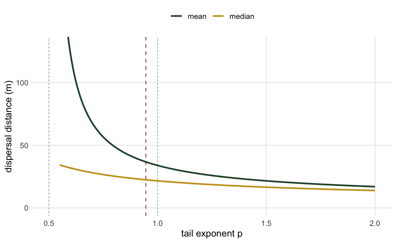
Corrected 1 October 2026: the figure’s alt text still called the median curve nearly flat, and now says it falls gently, far less steeply than the mean; the median’s coefficient of variation was called a bootstrap one, and is now described as its spread across the bootstrap exponents with the scale held at its fitted value.
Corrected 30 September 2026: the figure caption said the median barely moves and the text called it a flat function of the tail exponent; both now say it changes far less than the mean.
Ask how far a species disperses and the answer usually comes back as one number: the mean dispersal distance. It goes into spread-rate formulas, into connectivity metrics, into comparisons across species. It is also, for the fat-tailed kernels that dispersal data tend to favour, one of the least trustworthy numbers you can compute, because the mean is an average over the entire tail, including the part no trap ever caught. This tutorial takes the mean apart.
The mean lives in the tail
Start from the 2Dt kernel, whose distance density and survival function are
\[ k_D(r) = \frac{2p\,r}{a^2}\left(1 + \frac{r^2}{a^2}\right)^{-(p+1)}, \qquad P(R > r) = \left(1 + \frac{r^2}{a^2}\right)^{-p}. \]
The tail falls like a power law, \(r^{-(2p+1)}\), and the exponent \(p\) controls how heavy it is. That exponent also decides whether the mean and variance exist at all. Working through the integrals, the mean \(\int_0^\infty r\,k_D(r)\,dr\) is finite only when \(p > 1/2\), and the variance only when \(p > 1\). Below those thresholds the moment is infinite: not large, infinite.
The fitted kernel has p = 0.95 and scale 21.6 m. The seeds have a sample median of 22.1 m, a sample mean of 35.6 m, and a single furthest seed at 692 m. The mean sits well above the median because the far seeds pull it up. The fitted p of 0.95 is what decides which moments the fitted kernel has at all: the mean is finite only above 1/2, the variance only above 1.
How sensitive is the mean to that exponent? Hold the fitted scale fixed and vary p.
p_grid <- c(0.6, 0.7, 0.85, 1.0, 1.5)
mean_grid <- sapply(p_grid, function(pp) m_2dt(f$a, pp))
med_grid  <- sapply(p_grid, function(pp) med_2dt(f$a, pp))
names(mean_grid) <- names(med_grid) <- p_grid
mean_span <- max(mean_grid) / min(mean_grid)
med_span  <- max(med_grid) / min(med_grid)
Across that range the mean of the fitted kernel runs from 122 m down to 22 m, a factor of 5.7, and it heads to infinity as p approaches 1/2. The median moves from 32 m to 17 m over the same range, a factor of only 1.9, and it stays finite everywhere. The mean is a tail quantity; the median is a bulk quantity.
Not just sensitive: a poorly resolved exponent
Sensitivity to p would be harmless if p were pinned down. It is not. Bootstrap the fit and look at where the tail exponent lands.
set.seed(3033)
B <- 400
bfit <- replicate(B, { rs <- sample(r, n, replace = TRUE)   # refit both parameters on each resample
                       tryCatch(unlist(fit_2dt(rs)), error = function(e) c(a = NA_real_, p = NA_real_)) })
keep <- is.finite(bfit["p", ]) & bfit["p", ] < 50   # is.finite is not enough: drop the rare resample where the optimiser fails to converge and the tail exponent runs off to a huge (but finite) value
bp <- bfit["p", keep]; ba <- bfit["a", keep]
p_ci <- quantile(bp, c(0.025, 0.975))
frac_infvar <- mean(bp <= 1)     # fraction of fits with infinite variance
med_boot <- sapply(bp, function(pp) med_2dt(f$a, pp))
cv_med   <- 100 * sd(med_boot) / mean(med_boot)
mean_boot <- sapply(bp, function(pp) m_2dt(f$a, pp))   # the mean, scale held fixed as in the figure
cv_mean   <- 100 * sd(mean_boot) / mean(mean_boot)
cor_ap    <- cor(ba, bp)                                # refitted scale against refitted exponent
mean_refit <- mapply(m_2dt, ba, bp)                     # both parameters refitted
med_refit  <- mapply(med_2dt, ba, bp)
cv_mean_refit <- 100 * sd(mean_refit) / mean(mean_refit)
cv_med_refit  <- 100 * sd(med_refit) / mean(med_refit)
The tail exponent’s 95% bootstrap interval runs from 0.82 to 1.18, and 70 per cent of the resampled fits fall below p = 1, the value where the variance stops existing. For those fits the standard error of the mean dispersal distance is not a well-defined quantity to begin with. With the scale held at its fitted value, as in the figure above, that poorly resolved exponent moves the mean much more than the median: across the bootstrap exponents the mean’s coefficient of variation is 13 per cent, against a tame 6 per cent for the median. A refit does not hold the scale fixed. The refitted scale moves with the exponent (their correlation across the resamples is 0.89) and offsets much of the change, so with both parameters refitted the coefficient of variation of the fitted kernel’s mean drops to 7 per cent, and the median’s to 4 per cent. With this many seeds from the right kernel family, the fitted kernel’s mean is less precise than the median but not unresolved; what the data leave open is whether the variance exists at all.
When the mean does not exist at all
The sharpest version of the problem is easy to miss, because the software never complains. Simulate from a heavier tail, p = 0.45, for which the population mean is infinite.
set.seed(21)
r_heavy <- 20 * sqrt((1 - runif(2000))^(-1 / 0.45) - 1)   # 2Dt, p = 0.45: population mean does not exist
pop_mean <- m_2dt(20, 0.45)          # analytic population mean
stopifnot(is.infinite(pop_mean))     # it is infinite
emp_mean <- mean(r_heavy)            # sample mean: a finite number
emp_med  <- median(r_heavy)
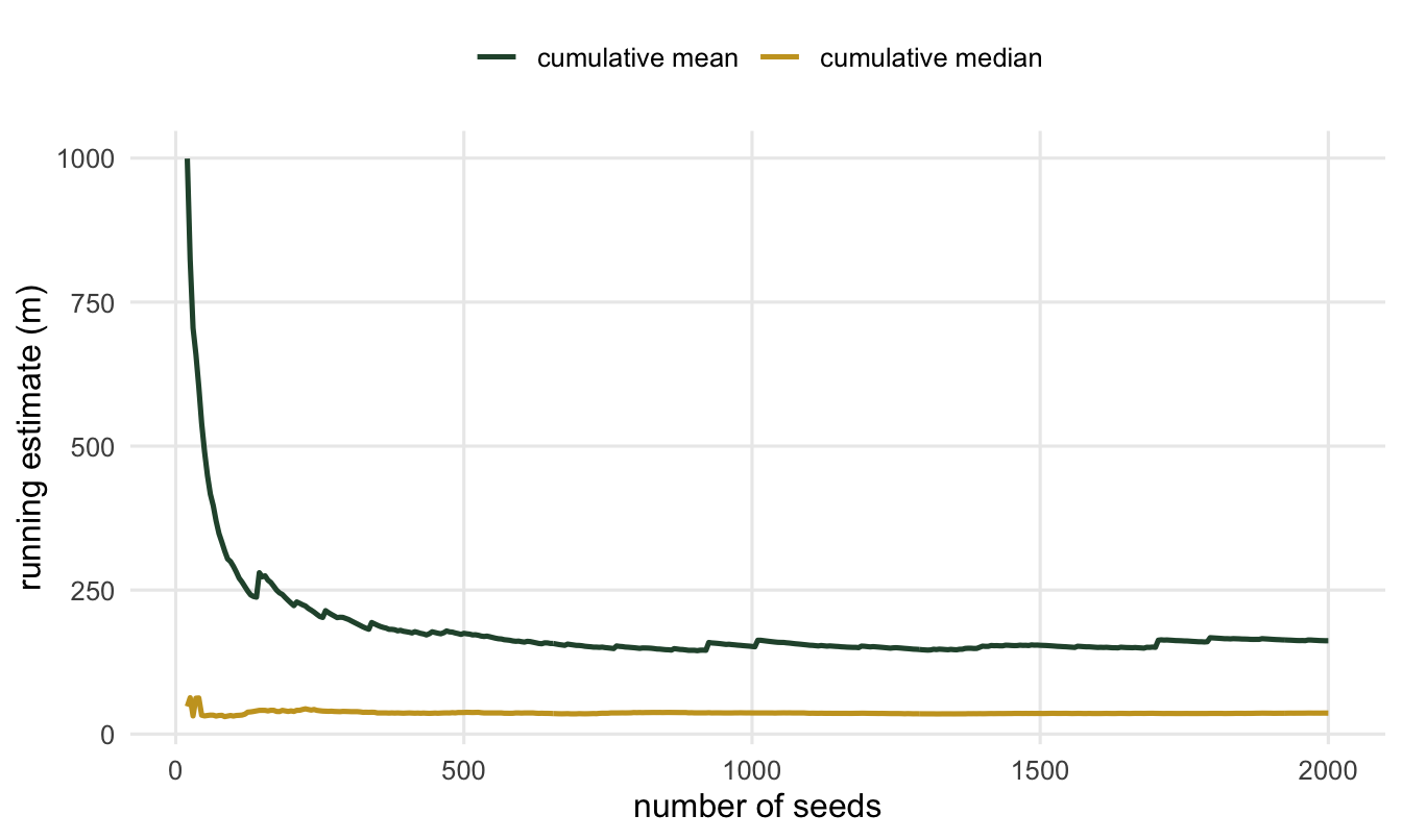
The population mean is infinite. The sample mean of two thousand draws is 249 m: a finite, ordinary-looking number that an analysis would report without hesitation, and that estimates nothing, because there is nothing finite to estimate. Draw a new sample and it lands somewhere else entirely, with no tendency to settle. The median, by contrast, is 41 m and behaves. The lesson is not that dispersal means are always infinite; it is that a finite sample mean is no evidence that the population mean exists.
The running average makes this visible. For the heavy-tailed data the cumulative mean lurches upward each time a new record-far seed arrives and never converges; the cumulative median walks steadily to its limit.
What to report
The median dispersal distance, or a fixed within-data quantile such as the distance containing 90 per cent of seeds, is anchored to the bulk of the data and stays stable whether the tail is thin or fat. The mean is not: it averages over a tail the traps barely sampled, it is less precise than the median even when the kernel family is right, and for a genuinely heavy kernel it does not exist while still returning a plausible number. Report the mean if a spread model needs it, but report it with the tail exponent beside it and treat it as a modelled extrapolation, not a measurement. The final tutorial in this cluster turns these observations into a short set of checks you can run on any fitted kernel.
References
Kot M, Lewis MA, van den Driessche P 1996. Ecology 77(7):2027-2042 (10.2307/2265698).
Clark JS 1998. American Naturalist 152(2):204-224 (10.1086/286162).
Nathan R, Klein E, Robledo-Arnuncio JJ, Revilla E 2012. In: Clobert J et al. (eds) Dispersal Ecology and Evolution, Oxford University Press, pp 187-210. ISBN 978-0-19-960889-8.