Fitting dispersal kernels in R

Seed-trap distances are not the dispersal kernel. Fitting a 2D dispersal kernel to distance data in R, and why the missing ring-area factor doubles the scale.

A dispersal kernel is a probability density: where does a seed (or a spore, or a juvenile) end up relative to its source? Almost every question that follows from it (how fast a population spreads, how far genes travel, how connected two patches are) reads off that density. So the first practical task is to fit one to data, and the most common data are seed-trap counts: traps placed at known distances from a source, each catching some seeds.

There is a trap hiding in that sentence, and it is geometric rather than statistical. The quantity you usually want is the location kernel: a density per unit area, describing how many seeds land on a small patch of ground at position (x, y). What a seed trap measures is a distance: how far a seed travelled, ignoring direction. Those are two different densities, and confusing them biases everything downstream.

Two densities, one process

For an isotropic kernel (no preferred direction), the location density depends only on the distance r from the source. Call it f(r): seeds per unit area at distance r. Because it is a density over the two-dimensional plane, it normalises with the area element, and the area of the thin ring at distance r grows with r:

\[ \int_0^\infty f(r)\, 2\pi r \, dr = 1 . \]

The density of the distance itself is therefore not f(r). It is the location density times the circumference of the ring the seed could have landed on:

\[ k_D(r) = 2\pi r \, f(r) . \]

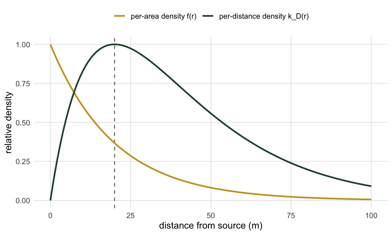
That factor of 2\pi r is the whole story. It is zero at the source and grows linearly, so even when the per-area density f(r) falls monotonically from a peak at the source, the per-distance density k_D(r) starts at zero, rises, and only then falls. The distance histogram peaks away from the source not because seeds prefer to travel that far, but because there is more ground at that distance.

Take the two-dimensional exponential kernel, a standard choice. Its location density and the distance density it implies are

\[ f(r) = \frac{1}{2\pi a^2}\, e^{-r/a}, \qquad k_D(r) = \frac{r}{a^2}\, e^{-r/a}, \]

so the distances follow a Gamma distribution with shape 2 and scale a. Let us simulate a seed rain from this kernel and look at both densities on the same axis.

# Distance density k_D(r) = 2*pi*r*f(r) for the 2D exponential location kernel.
# Sampling: the distance r ~ Gamma(shape = 2, scale = a).
kd_exp <- function(r, a) (r / a^2) * exp(-r / a)          # per-distance density
f_area <- function(r, a) (1 / (2 * pi * a^2)) * exp(-r / a) # per-area location density

set.seed(101)
a_true <- 20        # location scale, in metres
n_seed <- 400
r <- rgamma(n_seed, shape = 2, scale = a_true)            # observed distances

mean_r <- mean(r)
mode_kd <- a_true   # mode of Gamma(2, a) is (shape - 1) * scale = a

The seeds travel a mean distance of 40.3 m, close to the kernel mean of 2a = 40 m. The distance density peaks at 20 m, exactly one location-scale out. Neither number is the location scale of 20 m, and that gap is where the confusion begins.

Figure 1: The per-area location density falls monotonically from the source, but the per-distance density (location density times the ring circumference) peaks one location-scale out. The rise is geometry, not a dispersal preference. Both curves are scaled to a common height for comparison.

Fitting it, right and wrong

Now fit the kernel to the distances. The right way uses the distance density k_D(r), so the ring factor is built in. A common shortcut treats the distances as if they were exponentially distributed on their own, (1/b)\,e^{-r/b}, because “dispersal declines exponentially with distance” sounds reasonable. It is not reasonable: no two-dimensional dispersal process can produce exponentially distributed distances, because the distance density always carries the 2\pi r factor and so is always zero at the source. Fit both by maximum likelihood and compare.

# Correct: distances follow k_D(r) = (r/a^2) exp(-r/a), i.e. Gamma(shape 2, scale a).
nll_correct <- function(la) -sum(log(kd_exp(r, exp(la))))
a_hat <- exp(optimize(nll_correct, c(-5, 10))$minimum)

# Naive: treat distances as exponential with density (1/b) exp(-r/b).
nll_naive <- function(lb) -sum(dexp(r, rate = 1 / exp(lb), log = TRUE))
b_hat <- exp(optimize(nll_naive, c(-5, 10))$minimum)

ratio <- b_hat / a_hat

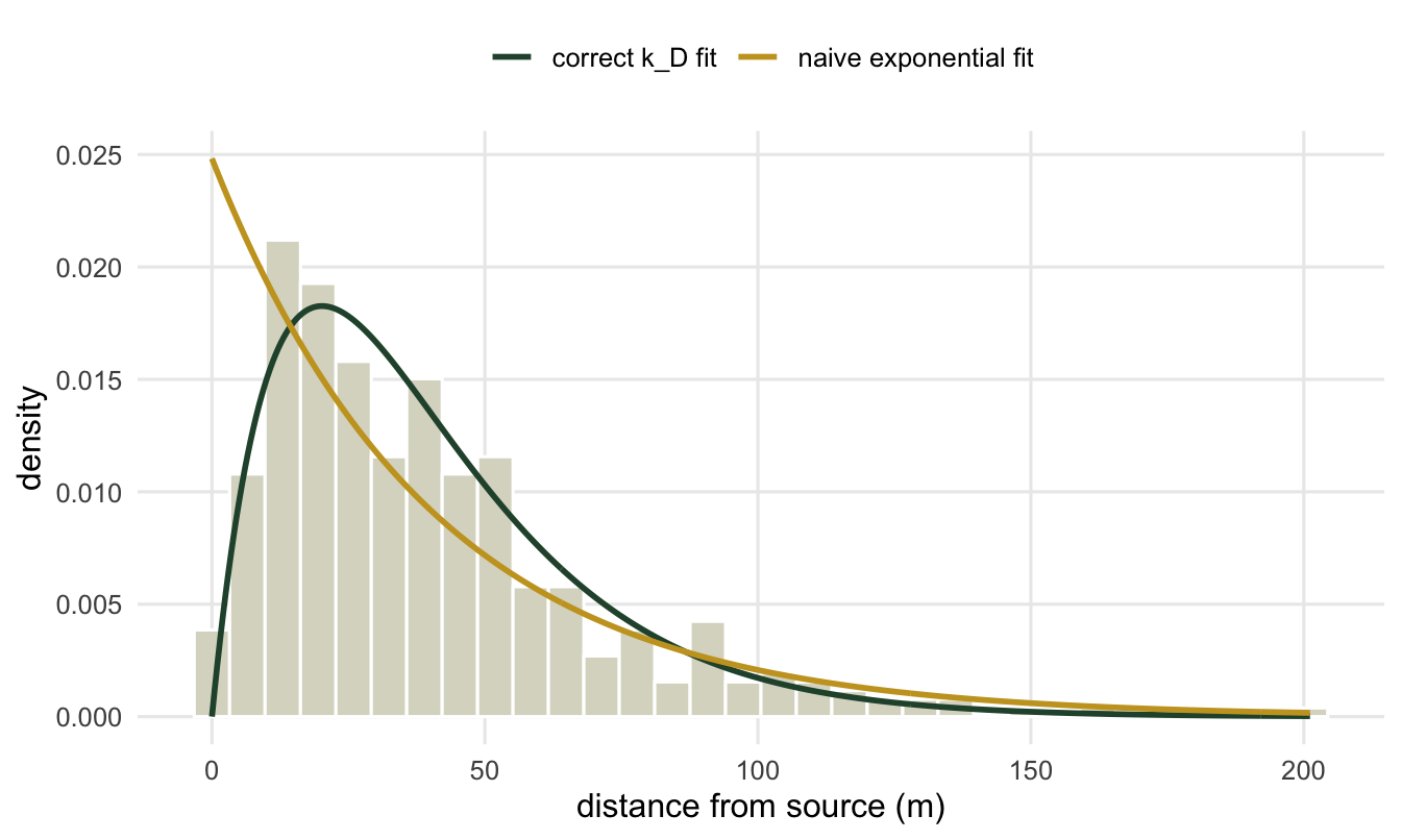
The correct fit recovers a location scale of 20.1 m, essentially the true 20 m. The naive fit reports 40.3 m, a factor of 2.00 too large. The reason is exact rather than a sampling accident: the maximum-likelihood scale of a Gamma with shape 2 is the sample mean divided by two, while the maximum-likelihood scale of an exponential is the sample mean itself. Ignore the ring factor and you double the scale, every time.

The scale is only half of it. The naive model also gets the shape wrong. Its density is monotone, so it claims most seeds land right next to the source and the number thins out steadily. The real distance density rises to a peak at 20 m. A reader who fits the exponential and plots it against the trap counts will see a curve that misses the hump entirely.

Figure 2: The observed distances (histogram) against the two fitted densities. The correctly fitted kernel reproduces the peak; the naive exponential is monotone and sits at twice the scale, missing both the shape and the location scale.

What to carry forward

The seed trap does not hand you the dispersal kernel. It hands you distances, and turning distances back into a kernel means dividing out the ring area, or equivalently fitting the distance density 2\pi r\,f(r) rather than f(r). Skip that step and two things go wrong at once: the estimated scale is too large (exactly double for the exponential), and the estimated shape loses the geometric peak that any real dispersal process must show.

The honest limit here is narrow but worth stating: fitting the right density recovers the scale cleanly when the kernel family is correct and the traps sample the whole distance range. Neither assumption is safe. The exponential is a thin-tailed choice, and the next tutorial shows that swapping it for a fat-tailed kernel leaves the near-source fit almost unchanged while moving the far tail by orders of magnitude. That tail is where long-distance dispersal lives, and it is where a dispersal analysis is most fragile.

References

Cousens R, Dytham C, Law R 2008. Dispersal in Plants: A Population Perspective. Oxford University Press. ISBN 978-0-19-929911-9.

Nathan R, Klein E, Robledo-Arnuncio JJ, Revilla E 2012. In: Clobert J et al. (eds) Dispersal Ecology and Evolution, Oxford University Press, pp 187-210. ISBN 978-0-19-960889-8.

Bullock JM, Mallada Gonzalez L, Tamme R, Gotzenberger L, White SM, Partel M, Hooftman DAP 2017. Journal of Ecology 105(1):6-19 (10.1111/1365-2745.12666).

Related tutorials

• Fat-tailed dispersal kernels
• The mean dispersal distance
• Checking a dispersal kernel
• Nonlinear regression with nls