Fitting a body size spectrum

Log bins shift the fitted size spectrum exponent by exactly one, and the likelihood never sees a bin. Fitting individual body mass data in R, no histogram.

Weigh every individual in a benthic sample and the masses span four or five orders of magnitude, with thousands of tiny animals and a handful of large ones. The standard summary of that spread is the size spectrum: a claim that the number of individuals at mass m falls off as a power of m, and a single exponent that says how fast.

The exponent gets compared across sites, across years and against fishing pressure, so it matters that two people analysing the same sample arrive at the same number. They frequently do not, and the reason is rarely the ecology. It is that the exponent depends on whether the counts were divided by the width of the bin they fell in, on how many bins there were, and on where the smallest mass in the fit was set. None of those is a property of the animals.

This post separates the three. The bin width turns out to shift the fitted slope by exactly one, the number of bins turns out to bias it in a direction that can be measured, and the maximum likelihood estimator turns out not to need bins at all.

A sample of individual masses

Individual dry masses in milligrams, drawn from a bounded power law so that the answer is known. The density is proportional to m^b between a lower and an upper mass, and b is the quantity every method below is trying to recover.

library(ggplot2)
library(patchwork)

te_paper  <- "#f5f4ee"
te_ink    <- "#16241d"
te_body   <- "#2c3a31"
te_forest <- "#275139"
te_rust   <- "#b5534e"
te_gold   <- "#c9b458"
te_line   <- "#dad9ca"

theme_datasheet <- function() {
  theme_minimal(base_size = 12) +
    theme(plot.background  = element_rect(fill = te_paper, colour = NA),
          panel.background = element_rect(fill = te_paper, colour = NA),
          panel.grid.major = element_line(colour = te_line, linewidth = 0.3),
          panel.grid.minor = element_blank(),
          text             = element_text(colour = te_body),
          plot.title       = element_text(colour = te_ink, face = "bold"),
          plot.subtitle    = element_text(colour = te_body),
          axis.text        = element_text(colour = te_body))
}

rbounded_pareto <- function(n, b, lo, hi) {
  u <- runif(n)
  ((hi^(b + 1) - lo^(b + 1)) * u + lo^(b + 1))^(1 / (b + 1))
}

b_true <- -2.05
m_lo   <- 0.5
m_hi   <- 8000
n_ind  <- 1200

set.seed(11)
mass <- rbounded_pareto(n_ind, b_true, m_lo, m_hi)
mass_max <- max(mass)

The sample holds 1200 individuals between 0.50 and 285 milligrams. Nothing in the analysis below uses b_true again until the end.

The bin width is not a plotting choice

Bins that double in width are the convention, because equal bins on the arithmetic scale put almost every animal in the first one. The bookkeeping question is what goes on the vertical axis: the raw count in each doubling class, or that count divided by the width of the class.

brk <- 2^(floor(log2(m_lo)):ceiling(log2(mass_max)))
cls <- cut(mass, brk, right = FALSE)

bm_in <- as.numeric(tapply(mass, cls, sum))
bm_in[is.na(bm_in)] <- 0

sp <- data.frame(
  lower   = brk[-length(brk)],
  upper   = brk[-1],
  n_in    = as.numeric(table(cls)),
  biomass = bm_in
)
sp$width <- sp$upper - sp$lower
sp$mid   <- sqrt(sp$lower * sp$upper)
sp$dens  <- sp$n_in / sp$width
sp       <- sp[sp$n_in > 0, ]

fit_count <- lm(log(n_in) ~ log(mid), data = sp)
fit_dens  <- lm(log(dens) ~ log(mid), data = sp)

slope_count <- unname(coef(fit_count)[2])
slope_dens  <- unname(coef(fit_dens)[2])
slope_shift <- slope_count - slope_dens
n_bin_used  <- nrow(sp)

The two lines are fitted to the same 10 bins holding the same 1200 animals. Counting gives a slope of -0.990. Dividing by bin width gives -1.990. The gap between them is 1.0000, and it is not approximately one, it is one.

The reason is that a doubling class starting at mass a has width a, so its width is proportional to its own position on the axis. Dividing the count by a subtracts log(a) from the vertical coordinate while the horizontal coordinate stays at log(a), which tilts the whole line by exactly one unit of slope. Any binning scheme with widths proportional to mass does this; the factor is a property of the bins, not of the sample.

pl <- ggplot(sp, aes(mid, n_in)) +
  geom_point(colour = te_forest, size = 2.4) +
  geom_smooth(method = "lm", formula = y ~ x, se = FALSE,
              colour = te_rust, linewidth = 0.7) +
  scale_x_log10() + scale_y_log10() +
  labs(x = "body mass (mg)", y = "individuals in class",
       title = "Counts per class",
       subtitle = sprintf("fitted slope %.2f", slope_count)) +
  theme_datasheet()

pr <- ggplot(sp, aes(mid, dens)) +
  geom_point(colour = te_forest, size = 2.4) +
  geom_smooth(method = "lm", formula = y ~ x, se = FALSE,
              colour = te_rust, linewidth = 0.7) +
  scale_x_log10() + scale_y_log10() +
  labs(x = "body mass (mg)", y = "individuals per mg",
       title = "Counts per unit mass",
       subtitle = sprintf("fitted slope %.2f", slope_dens)) +
  theme_datasheet()

pl + pr + plot_annotation(theme = theme_datasheet())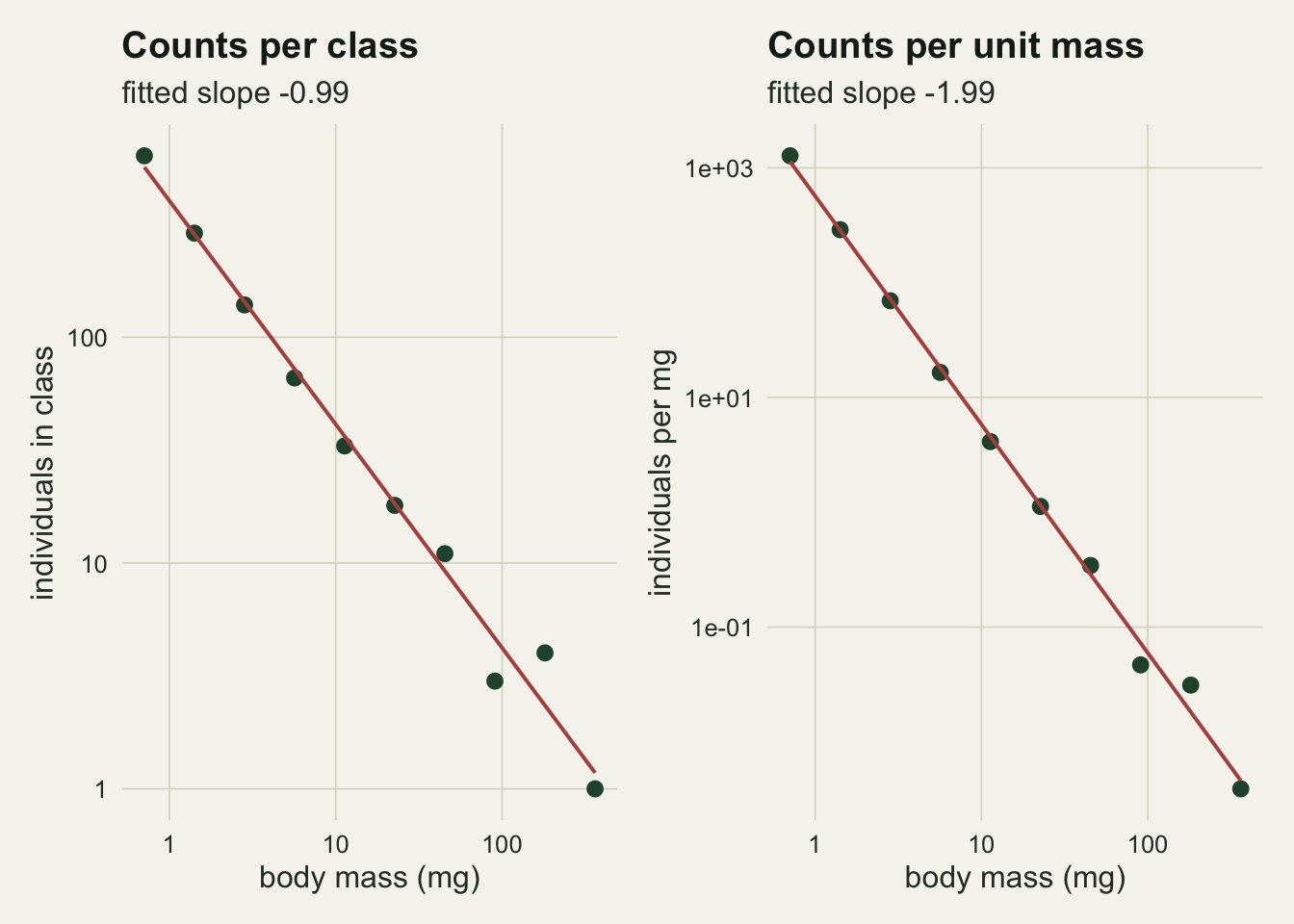

Figure 1: One sample of individual masses, binned once, plotted two ways.

This is the same bookkeeping that trips up dispersal kernels, where the density of distances carries a ring area that the density of positions does not, and the same failure to divide by the width of the measure produces a scale parameter that is wrong by a fixed factor.

The bookkeeping continues into biomass. Total mass in a doubling class rises one further power of m above the count, and dividing that by class width takes one back off, so four quantities from one sample give four different slopes.

slope_bm      <- unname(coef(lm(log(biomass) ~ log(mid), data = sp))[2])
slope_bm_dens <- unname(coef(lm(log(biomass / width) ~ log(mid), data = sp))[2])

Counts give -0.99, counts per unit mass give -1.99, biomass gives -0.02 and biomass per unit mass gives -1.02. A published slope near -1 and a published slope near -2 can describe an identical sample. The number is uninterpretable without the sentence that says which of the four it is, and that sentence is missing from a lot of papers.

The likelihood never sees a bin

If the masses really do follow a power law above some lower limit, the exponent has a closed form. Writing the density as proportional to m^b with b below minus one, and setting alpha = -b, the maximum likelihood estimate from n observed masses above a lower limit m0 is a single expression, and so is its standard error.

pareto_alpha <- function(x, m0) 1 + length(x) / sum(log(x / m0))

alpha_hat <- pareto_alpha(mass, m_lo)
b_hat     <- -alpha_hat
alpha_se  <- (alpha_hat - 1) / sqrt(length(mass))

nll_bounded <- function(b, x, lo, hi) {
  -sum(log((b + 1) * x^b / (hi^(b + 1) - lo^(b + 1))))
}
b_bounded <- optimize(nll_bounded, c(-4, -1.01),
                      x = mass, lo = m_lo, hi = m_hi)$minimum

The estimate is -2.049 with a standard error of 0.030, against a truth of -2.05. Allowing for the upper bound leaves it at -2.049: the largest animal in the tray sits far below the bound, so that refinement has nothing to correct here.

Two things are worth noticing about that expression. It contains no bins, no midpoints and no regression, so the choice of doubling class or decade class or any other class cannot influence it. And it is the same estimator that sits behind the generalised Pareto fit used for extremes: a Pareto tail is a generalised Pareto with the scale tied to the threshold, and alpha is the reciprocal of the shape parameter.

What the bins cost

Comparing estimators needs repetition rather than one sample, so here are four hundred fresh samples at two sample sizes, each fitted by the closed form and by a log-binned regression at three bin counts.

n_rep <- 400

binned_b <- function(x, m0, n_bin) {
  bb <- exp(seq(log(m0), log(max(x) * 1.0001), length.out = n_bin + 1))
  ct <- as.numeric(table(cut(x, bb, right = FALSE)))
  wd <- diff(bb)
  md <- sqrt(bb[-length(bb)] * bb[-1])
  keep <- ct > 0
  unname(coef(lm(log(ct[keep] / wd[keep]) ~ log(md[keep])))[2])
}

n_small <- 200
bin_grid <- c(6, 10, 20)

set.seed(202)
sweep_one <- function(n_draw) {
  out <- t(replicate(n_rep, {
    x <- rbounded_pareto(n_draw, b_true, m_lo, m_hi)
    c(-pareto_alpha(x, m_lo), vapply(bin_grid, function(k) binned_b(x, m_lo, k), 0))
  }))
  colnames(out) <- c("likelihood", paste0("bins", bin_grid))
  data.frame(
    method = colnames(out),
    n_draw = n_draw,
    bias   = colMeans(out) - b_true,
    rmse   = sqrt(colMeans((out - b_true)^2)),
    mc_se  = apply(out, 2, sd) / sqrt(n_rep),
    row.names = NULL
  )
}
mc <- rbind(sweep_one(n_small), sweep_one(n_ind))

mle_rmse_small <- mc$rmse[mc$method == "likelihood" & mc$n_draw == n_small]
b20_rmse_small <- mc$rmse[mc$method == "bins20"     & mc$n_draw == n_small]
b20_bias_small <- mc$bias[mc$method == "bins20"     & mc$n_draw == n_small]
b06_bias_small <- mc$bias[mc$method == "bins6"      & mc$n_draw == n_small]
mle_bias_big   <- mc$bias[mc$method == "likelihood" & mc$n_draw == n_ind]
b20_bias_big   <- mc$bias[mc$method == "bins20"     & mc$n_draw == n_ind]
rmse_ratio     <- b20_rmse_small / mle_rmse_small
mc_se_max      <- max(mc$mc_se)
b06_bias_big   <- mc$bias[mc$method == "bins6"  & mc$n_draw == n_ind]
b10_bias_big   <- mc$bias[mc$method == "bins10" & mc$n_draw == n_ind]
bin_gap_big    <- b10_bias_big - b06_bias_big

The closed form is essentially unbiased at both sample sizes, with a bias of -0.002 at 1200 individuals. Every binned fit is biased towards a shallower spectrum, the bias grows with the number of bins rather than shrinking, and at 200 individuals the twenty bin version is off by +0.245 on average with a root mean squared error 3.5 times the likelihood’s.

mc$method <- factor(mc$method, levels = c("likelihood", paste0("bins", bin_grid)),
                    labels = c("likelihood", sprintf("%d bins", bin_grid)))
mc$label  <- factor(ifelse(mc$n_draw == n_small,
                           sprintf("%d individuals", n_small),
                           sprintf("%d individuals", n_ind)))

pa <- ggplot(mc, aes(method, bias, colour = label, group = label)) +
  geom_hline(yintercept = 0, colour = te_line, linewidth = 0.6) +
  geom_line(linewidth = 0.6) + geom_point(size = 2.6) +
  scale_colour_manual(values = c(te_forest, te_rust), name = NULL) +
  labs(x = NULL, y = "bias in b", title = "Binning biases the exponent upwards") +
  theme_datasheet() + theme(legend.position = "none")

pb <- ggplot(mc, aes(method, rmse, colour = label, group = label)) +
  geom_line(linewidth = 0.6) + geom_point(size = 2.6) +
  scale_colour_manual(values = c(te_forest, te_rust), name = NULL) +
  labs(x = NULL, y = "root mean squared error", title = "And it costs precision as well") +
  theme_datasheet() + theme(legend.position = "bottom")

pa / pb + plot_annotation(theme = theme_datasheet())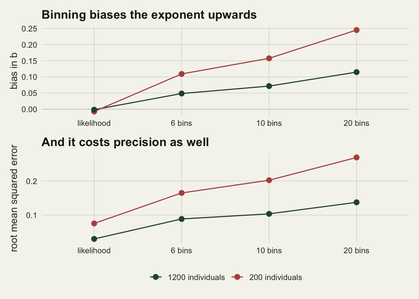

Figure 2: Bias and error of four estimators of the spectrum exponent, over 400 samples.

The mechanism sits in the top bins. Under the truth, the expected count in the largest classes of a small sample is below one, and a bin cannot hold a fraction of an animal. It either holds none, in which case the logarithm is undefined and the bin is dropped, or it holds at least one, in which case it stands above where the line should pass.

expected_in <- function(bb, n_draw) {
  n_draw * (bb[-1]^(b_true + 1) - bb[-length(bb)]^(b_true + 1)) /
    (m_hi^(b_true + 1) - m_lo^(b_true + 1))
}

set.seed(21)
floor_stat <- replicate(n_rep, {
  x  <- rbounded_pareto(n_small, b_true, m_lo, m_hi)
  bb <- exp(seq(log(m_lo), log(max(x) * 1.0001), length.out = 11))
  ct <- as.numeric(table(cut(x, bb, right = FALSE)))
  ex <- expected_in(bb, n_small)
  thin <- ex < 1
  c(sum(thin), sum(ct[thin] > 0),
    if (any(thin & ct > 0)) mean(ct[thin & ct > 0] / ex[thin & ct > 0]) else NA_real_)
})

thin_bins  <- mean(floor_stat[1, ])
thin_kept  <- mean(floor_stat[2, ])
thin_ratio <- mean(floor_stat[3, ], na.rm = TRUE)

Across the four hundred small samples, an average of 1.7 of the ten bins expect fewer than one animal, 1.2 of them survive into the regression, and those survivors carry on average 5.0 times the count the truth calls for. They sit at the far right of the horizontal range, where a point pulls hardest on a slope, and they can only ever be too high. Adding bins adds more of them, which is why the bias grew rather than shrank.

Where the spectrum starts

The lower limit is the remaining knob, and it is the one that moves the answer furthest. Gear misses small animals: a sieve, a net or a sorter retains large individuals reliably and small ones erratically, so the observed distribution rolls over at the bottom even when the underlying one does not.

n_pool     <- 300000
m_pool_lo  <- 0.05
retain_50  <- 1.5
retain_sd  <- 0.4

set.seed(1)
pool     <- rbounded_pareto(n_pool, b_true, m_pool_lo, m_hi)
p_retain <- 1 / (1 + exp(-(log(pool) - log(retain_50)) / retain_sd))
caught   <- pool[runif(n_pool) < p_retain]

b_naive <- -pareto_alpha(caught, min(caught))

The retained sample holds 11424 individuals. Fitting the closed form from the smallest one in the tray gives -1.267 against a truth of -2.05, an error far larger than anything the binning produced. The estimator is doing exactly what it was asked; the request was wrong.

The usual repair is to fit above a lower limit chosen so that the part of the sample above it looks Pareto, measured by the Kolmogorov-Smirnov distance between the empirical distribution above the limit and the fitted one.

ks_pareto <- function(x, m0) {
  z <- sort(x[x >= m0])
  k <- length(z)
  a <- pareto_alpha(z, m0)
  theo <- 1 - (z / m0)^(-(a - 1))
  list(alpha = a, n_above = k,
       ks = max(abs(c(theo - (seq_len(k) - 1) / k, seq_len(k) / k - theo))))
}

n_grid  <- 60
min_fit <- 100
lo_q    <- 0.002
hi_q    <- 0.92
xmin_grid <- exp(seq(log(unname(quantile(caught, lo_q))),
                     log(unname(quantile(caught, hi_q))), length.out = n_grid))

scan_out <- do.call(rbind, lapply(xmin_grid, function(m0) {
  if (sum(caught >= m0) < min_fit) return(NULL)
  s <- ks_pareto(caught, m0)
  data.frame(xmin = m0, b = -s$alpha, ks = s$ks, n_above = s$n_above)
}))

pick     <- which.min(scan_out$ks)
xmin_ks  <- scan_out$xmin[pick]
b_ks     <- scan_out$b[pick]
n_above  <- scan_out$n_above[pick]
b_span   <- range(scan_out$b)

Minimising that distance picks a lower limit of 3.3 milligrams, keeps 3667 individuals and returns -2.054, which lands on the truth. The more useful output is the rest of the curve: across the whole grid of candidate limits the exponent runs from -1.29 to -2.10. That is a full unit of exponent, from one tray of animals, produced by moving one knob that the methods section usually does not mention.

ggplot(scan_out, aes(xmin, b)) +
  geom_hline(yintercept = b_true, colour = te_gold, linetype = "dashed",
             linewidth = 0.7) +
  geom_vline(xintercept = xmin_ks, colour = te_rust, linetype = "dashed",
             linewidth = 0.7) +
  geom_line(colour = te_forest, linewidth = 0.9) +
  scale_x_log10() +
  labs(x = "lower mass limit of the fit (mg)", y = "fitted exponent b",
       title = "One tray of animals, one unit of exponent",
       subtitle = sprintf("dashed gold: truth %.2f; dashed red: KS limit %.1f mg",
                          b_true, xmin_ks)) +
  theme_datasheet()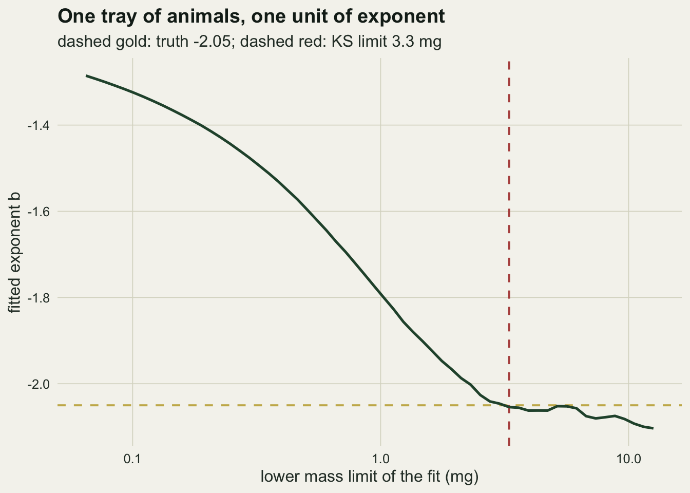

Figure 3: Fitted exponent against the lower mass limit, with the limit chosen by minimum KS distance.

Choosing a lower limit this way is the same operation as choosing a threshold for a generalised Pareto fit to extremes, with the same character: the criterion is a rule for picking, not evidence that the pick is right. The curve above is the honest report, and a single number pulled off it is not.

What to report

Say which spectrum the exponent belongs to. Counts per class, counts per unit mass, biomass per class and biomass per unit mass differ by whole units of slope, and a value quoted without that label cannot be compared with anything.

Fit by likelihood, not by regression on binned counts. The closed form is one line, it has a standard error that is another line, and the four hundred replicate comparison above shows it beating every binned alternative on bias and on error at both sample sizes.

Give the lower mass limit, the number of individuals above it, and what the exponent does as the limit moves. The limit is where the real disagreement between analyses lives, and a sensitivity curve costs one plot.

If a binned figure is wanted, and it usually is, plot the binned spectrum and fit the likelihood. The two are not in competition once the line on the figure is drawn from the likelihood estimate rather than from a regression through the points.

Honest limits

The data here are generated from a power law, so every method is being scored on its ability to recover a truth that exists. Real body mass distributions are not exactly power laws, and when the shape is wrong the likelihood estimator is not saved by being efficient: it returns the exponent of the best fitting power law, which may describe nothing. Testing whether a power law is the right family at all is a separate exercise, and the site has covered how weak that kind of comparison can be when two families are close.

The Kolmogorov-Smirnov criterion for the lower limit is a heuristic with known failure modes. It tends to pick a limit that discards more data than necessary when the departure from a power law is mild, and it has no defence at all against a distribution that is curved throughout, where it will find a local stretch that looks straight. The flat section of the curve above is doing more of the work than the minimum is.

The selectivity example uses a smooth retention curve that reaches one well below the chosen limit, which is the favourable case. Gear whose retention is still climbing across the fitted range biases the exponent in a way no choice of lower limit can remove, because there is no mass above which the sample is a fair draw.

The upper end is left alone throughout. A bounded power law was simulated and an unbounded one was fitted, which costs little here because the largest observed mass sits far below the bound. Samples whose largest individuals press against a real physiological or gear-imposed ceiling need the bounded likelihood, and the difference is then not small.

Finally, 400 replicates give each bias a Monte Carlo standard error of at most 0.0063 on the scale of the exponent. That is below every gap discussed above, including the 0.023 between six and ten bins at the larger sample size, so the ordering is solid. The fourth decimal place of any one of them is not.

References

Edwards AM, Robinson JPW, Plank MJ, Baum JK, Blanchard JL 2017 Methods in Ecology and Evolution 8(1):57-67 (10.1111/2041-210X.12641)

White EP, Enquist BJ, Green JL 2008 Ecology 89(4):905-912 (10.1890/07-1288.1)

Clauset A, Shalizi CR, Newman MEJ 2009 SIAM Review 51(4):661-703 (10.1137/070710111)

Sheldon RW, Prakash A, Sutcliffe WH 1972 Limnology and Oceanography 17(3):327-340 (10.4319/lo.1972.17.3.0327)

Related tutorials

• Peaks over threshold and the GPD
• Allometry and log-log regression in R
• Fitting dispersal kernels in R
• Range size distributions