library(ggplot2)
library(patchwork)

te_paper  <- "#f5f4ee"
te_ink    <- "#16241d"
te_body   <- "#2c3a31"
te_forest <- "#275139"
te_rust   <- "#b5534e"
te_gold   <- "#c9b458"
te_line   <- "#dad9ca"

theme_datasheet <- function() {
  theme_minimal(base_size = 12) +
    theme(plot.background  = element_rect(fill = te_paper, colour = NA),
          panel.background = element_rect(fill = te_paper, colour = NA),
          panel.grid.major = element_line(colour = te_line, linewidth = 0.3),
          panel.grid.minor = element_blank(),
          text             = element_text(colour = te_body),
          plot.title       = element_text(colour = te_ink, face = "bold"),
          plot.subtitle    = element_text(colour = te_body),
          axis.text        = element_text(colour = te_body))
}Gill-net selectivity and the fish it cannot see
R
fisheries
sampling design
selectivity
simulation
ecology tutorial
Gill-net mesh series leave a blind zone that the SELECT correction cannot fill. Measuring the corrected share of large fish in R, and what one more mesh buys.
A lake monitoring programme sets a multi-mesh survey net overnight, measures every fish, and reports the length distribution of the perch population. The report carries two numbers the managers care about: the mean length, and the proportion of fish over 25 cm, which is the size at which the local anglers start keeping them. Both numbers come out of the catch, and both are wrong in a direction everybody in the room knows about: a gill net catches a fish whose girth fits the mesh, so a net made of 20, 25 and 31 mm bar mesh sees small and medium fish well and large fish hardly at all.
The standard repair is to estimate the selectivity curve from the catch itself. Because each mesh in the series fishes the same water at the same time, the lengths a 31 mm mesh catches relative to a 20 mm mesh contain information about the shape of the curve, and Millar turned that into a likelihood: condition on a fish of length L having been caught at all, and model which mesh caught it. The fitted curve then divides the pooled catch, class by class, and what comes out is presented as the population’s length distribution. This is the SELECT method; Millar and Holst give the gill-net and hook version with the family set used below, and it is what a lake survey report means when it says the size structure is selectivity-corrected.
The correction works where the gear works. This post measures what it does where the gear does not, which for a three-mesh series is exactly the length range the managers asked about.
The mechanism is not new on this site. Checking a dispersal kernel fits four kernel families to the same seed distances and finds that their fitted 90th percentiles agree closely while their probabilities of a seed passing 150 m differ by orders of magnitude; its conclusion is that a within-data quantile is a stable target and a far-tail probability is a property of the family you chose. Extrapolating a species-area curve beyond the plots makes the same point with a model comparison that picks the right-looking curve and still misses richness at the area that matters. The gill-net case would be a third costume for that mechanism, except for one thing: here the quantity the managers want is the tail. Reporting a within-data quantile instead is not an option, because the whole product is the share of large fish. So the interesting question is not whether the family decides the tail, which it does, but how much of the population the gear cannot see, and what fixes it.
The other close post is trawl selectivity when hauls differ, which fits retention curves to a covered-codend trial where every escaping fish is counted in a fine-meshed cover. That design has a control: the number of fish that entered the gear is known at every length, so retention is a binomial proportion and L50 is estimated directly. Its honest limits name the SELECT method and say that nothing in that post measures it. A gill-net series has no cover and no control. Selectivity and size structure come out of one catch table, and the division is an extrapolation wherever the largest mesh has stopped catching. Fitting a body size spectrum meets the same gear problem from the other side. It starts from a complete set of individual masses, thins the small ones with a logistic retention curve, and then asks where the spectrum can be started so that the part above the limit is a fair draw. The repair there is to throw the badly sampled part away, and it works because the quantity wanted, the exponent, lives in the part that is sampled well. Fishing, age truncation and spawning variability works from known ages, with fishing selectivity acting on survival rather than on the observation. Here the badly sampled part is the product, so neither repair is available.
A population, a mesh series, and a blind zone
The population is five cohorts of perch in 1 cm length classes from 8 to 40 cm. Mean lengths are 11, 17, 22.5, 27 and 30.5 cm, the within-cohort spread grows from 1.6 to 2.6 cm with age, and each cohort is half the size of the one before it, which is an annual survival of 0.5. Nothing here is fitted to data; these are design constants, chosen once and left alone.
The selectivity families are the ones Millar and Fryer set out in their review. All four are written as relative selectivity, because that is all a multi-mesh series can identify: the normal-scale curve of geometric similarity, where the mode and the spread both scale with mesh size; the lognormal; the gamma; and the bi-normal, which adds a second, wider component at a larger length to represent fish that are tangled or wedged rather than caught cleanly by the girth. The first three peak at exactly one and the bi-normal a little above one, because its second component adds to the first; the overall height never enters, since it cancels in the conditional likelihood and again when the corrected distribution is renormalised.
len      <- 8:40
coh_mu   <- c(11, 17, 22.5, 27, 30.5)
coh_sd   <- c(1.6, 1.9, 2.2, 2.4, 2.6)
coh_wt   <- 0.5^(0:4); coh_wt <- coh_wt / sum(coh_wt)
f_pop    <- rowSums(sapply(seq_along(coh_mu),
                           function(a) coh_wt[a] * dnorm(len, coh_mu[a], coh_sd[a])))
f_pop    <- f_pop / sum(f_pop)
big_cut  <- 25
is_big   <- len >= big_cut
truth_big  <- sum(f_pop[is_big])
truth_mean <- sum(len * f_pop)

sel_normal <- function(x, mesh, th) exp(-(x - th[1] * mesh)^2 / (2 * (th[2] * mesh)^2))
sel_lnorm  <- function(x, mesh, th) {
  mu <- log(th[1] * mesh)
  exp(mu - th[2]^2 / 2 - (log(x) - mu)^2 / (2 * th[2]^2)) / x
}
sel_gamma  <- function(x, mesh, th) {
  alpha <- th[2]; kk <- th[1] * mesh / (alpha - 1)
  (x / ((alpha - 1) * kk))^(alpha - 1) * exp(alpha - 1 - x / kk)
}
sel_binorm <- function(x, mesh, th)
  sel_normal(x, mesh, th[1:2]) + th[5] * sel_normal(x, mesh, th[3:4])

fams    <- list(normal = sel_normal, lognormal = sel_lnorm,
                gamma = sel_gamma, bimodal = sel_binorm)
th_true <- list(normal  = c(0.62, 0.09),
                bimodal = c(0.62, 0.09, 0.62 * 1.35, 0.09 * 1.6, 0.35))

mesh_three <- c(20, 25, 31)
mesh_four  <- c(20, 25, 31, 39)
blind_frac <- 0.10

summed_sel <- function(mesh, truth_fam)
  rowSums(outer(len, mesh, fams[[truth_fam]], th = th_true[[truth_fam]]))
blind_parts <- function(mesh, truth_fam, frac = blind_frac) {
  st   <- summed_sel(mesh, truth_fam); st <- st / max(st)
  peak <- len[which.max(st)]
  up   <- len > peak & st < frac
  down <- len < peak & st < frac
  c(upper = sum(f_pop[up]), lower = sum(f_pop[down]),
    total = sum(f_pop[up | down]), start = min(len[up]))
}

blind3_n <- blind_parts(mesh_three, "normal")
blind4_n <- blind_parts(mesh_four,  "normal")
blind3_b <- blind_parts(mesh_three, "bimodal")

st3 <- summed_sel(mesh_three, "normal"); st3 <- st3 / max(st3)
st4 <- summed_sel(mesh_four,  "normal"); st4 <- st4 / max(st4)
sel_at_25 <- st3[len == 25]; sel_at_30 <- st3[len == 30]
sel4_at_30 <- st4[len == 30]
The true share of fish at or above 25 cm is 0.1109 and the true mean length is 15.75 cm. Against the three-mesh series the summed relative selectivity at 25 cm is 0.071 of its maximum and at 30 cm it is 0.0003. Adding the 39 mm mesh lifts the 30 cm figure to 0.150.
Define the blind zone as the length classes where the summed relative selectivity of the whole series is below 10 per cent of its maximum. That threshold is a convention, fixed here before anything was run. Nothing in the fitting or in the correction uses it, so the simulation results in the rest of the post do not depend on it at all; the descriptive numbers in this section do depend on it, and by more than one might expect, which the sensitivity check below measures. What it buys is a single number for how much of the population the gear is effectively not sampling. A mesh series is blind at both ends, so the two sides are worth keeping apart: the small fish that swim through every panel, and the large fish that bounce off every panel.
Under the normal-scale truth the three-mesh series is blind above 25 cm, and that upper blind zone holds 0.1109 of the population, with 0.0223 more below the small end and 0.1332 in total. Adding the 39 mm panel moves the blind edge to 31 cm and drops the upper share to 0.0209.
The blind edge landing on the managers’ cut is a coincidence of this design, and the two numbers above should be read with that in mind. What is not a convention is the selectivity itself: the three-mesh series is at 0.071 of its peak at the cut and 0.0003 at 30 cm, so essentially the whole large-fish class sits where this series barely fishes. Where the edge is drawn, though, depends on both knobs.
edge_by_frac <- sapply(c(0.05, 0.10, 0.15), function(fr)
  blind_parts(mesh_three, "normal", fr)[c("start", "upper")])
colnames(edge_by_frac) <- c("5", "10", "15")
edge_by_mesh <- sapply(28:34, function(m)
  blind_parts(c(20, 25, m), "normal")[c("start", "upper")])
colnames(edge_by_mesh) <- as.character(28:34)

peak_ratio  <- max(summed_sel(mesh_three, "bimodal")) / max(summed_sel(mesh_three, "normal"))
peak_at_n   <- len[which.max(summed_sel(mesh_three, "normal"))]
peak_at_b   <- len[which.max(summed_sel(mesh_three, "bimodal"))]
small_abs_n <- summed_sel(mesh_three, "normal")[len == 12]
small_abs_b <- summed_sel(mesh_three, "bimodal")[len == 12]
tail_abs_n  <- summed_sel(mesh_three, "normal")[len == 30]
tail_abs_b  <- summed_sel(mesh_three, "bimodal")[len == 30]
Hold the mesh series and move the threshold: at 5 per cent of peak the blind zone starts at 26 cm and holds 0.0904 of the population, at 15 per cent it starts at 24 cm and holds 0.1348. Hold the threshold at 10 per cent and move the largest mesh instead: 24 cm at 30 mm, 25 cm at 31 mm, 26 cm at 32 mm and 27 cm at 33 mm. One millimetre of bar mesh is worth a centimetre of blind edge over that stretch, which is why the blind zone is a statement about a particular series and a particular convention rather than a property of gill nets.
Under the bi-normal truth the arithmetic changes at both ends, and the two ends change for different reasons. At the top the tangling component puts real catching power where the normal-scale curve had almost none: absolute summed selectivity at 30 cm is 0.2470 under the bi-normal truth against 0.0006 under the normal-scale one, so the three-mesh series is blind only above 31 cm, with 0.0209 of the population up there. At the small end nothing of the kind happens. The same second component lifts the peak of the summed curve by a factor of 1.31 and moves it from 14 to 17 cm, and measured against that higher peak the lower blind share rises from 0.0223 to 0.0817, which looks like the gear going blind at the small end and is not: absolute summed selectivity at 12 cm is 1.4182 under the bi-normal truth against 1.3090 under the normal-scale one, a little higher rather than lower. The small classes fall below the threshold because the yardstick got longer. This is the awkward part of a relative-selectivity definition: only ratios between meshes are identified, so a blind zone defined as a fraction of the peak moves whenever the peak moves.
blind_lo  <- as.numeric(blind3_n["start"])
band_lin  <- annotate("rect", xmin = blind_lo - 0.5, xmax = max(len) + 0.5,
                      ymin = -Inf, ymax = Inf, fill = te_rust, alpha = 0.10)
band_log  <- annotate("rect", xmin = blind_lo - 0.5, xmax = max(len) + 0.5,
                      ymin = 1e-3, ymax = 1, fill = te_rust, alpha = 0.10)

p_pop <- ggplot(data.frame(len = len, f = f_pop), aes(len, f)) + band_lin +
  geom_line(colour = te_forest, linewidth = 0.8) +
  labs(x = NULL, y = "population share", title = "Length distribution and what the gear sees") +
  theme_datasheet()

sel_long <- rbind(data.frame(len = len, s = st3, series = "three meshes (20/25/31)"),
                  data.frame(len = len, s = st4, series = "four meshes (20/25/31/39)"))
p_sel <- ggplot(sel_long, aes(len, pmax(s, 1e-3), colour = series)) + band_log +
  geom_hline(yintercept = blind_frac, linetype = "dashed", colour = te_body, linewidth = 0.35) +
  geom_line(linewidth = 0.8) +
  scale_y_log10(limits = c(1e-3, 1)) +
  scale_colour_manual(values = c("three meshes (20/25/31)" = te_rust,
                                 "four meshes (20/25/31/39)" = te_gold)) +
  labs(x = "length (cm)", y = "summed relative selectivity", colour = NULL) +
  theme_datasheet() + theme(legend.position = "bottom")

p_pop / p_sel + plot_layout(heights = c(1, 1.2)) +
  plot_annotation(theme = theme_datasheet())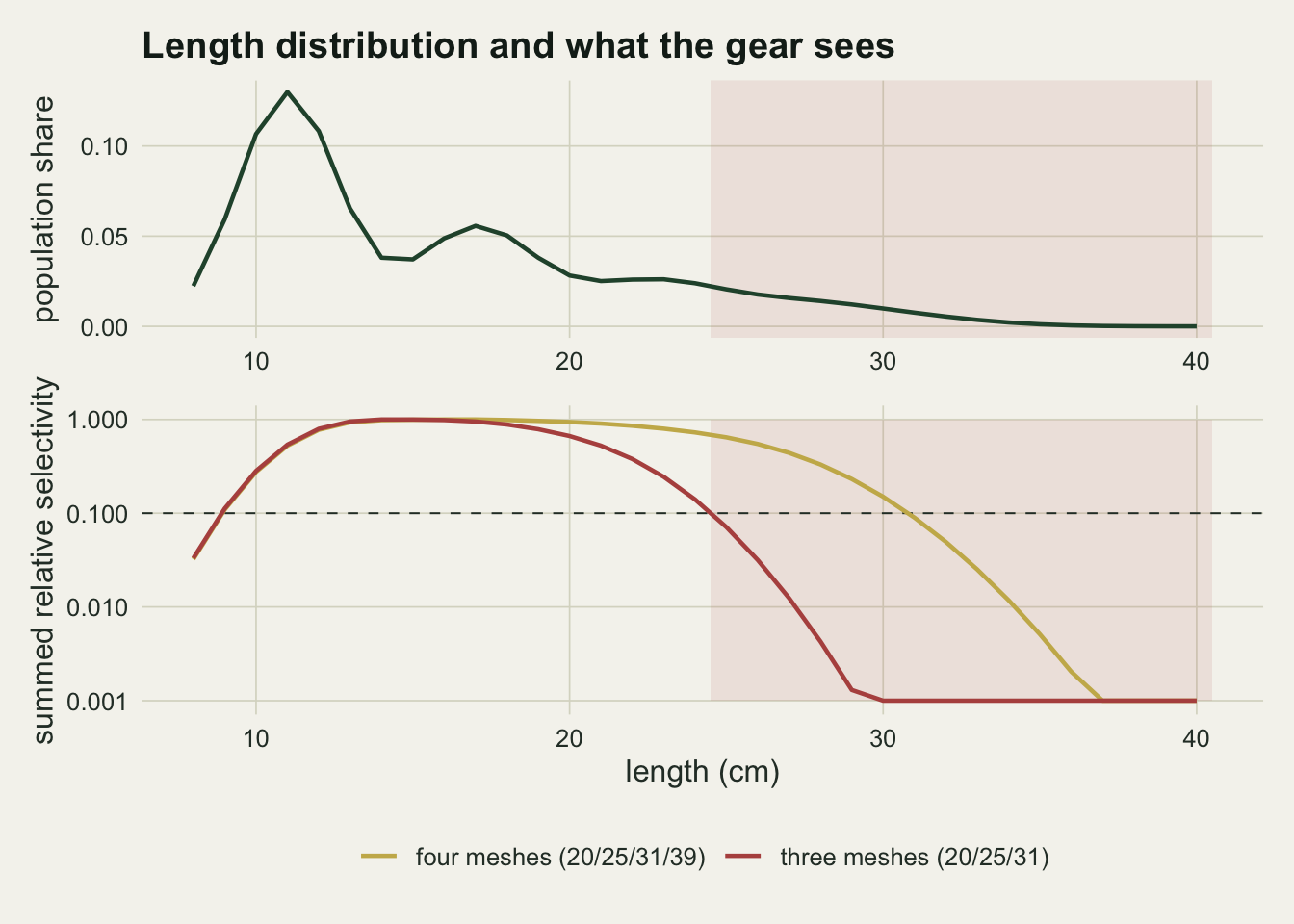
Two things in that figure are arithmetic and not findings, and it is worth saying so plainly before any simulation runs. First, given a known selectivity curve the raw catch share is a deterministic product: the expected catch in a length class is the population share times the summed selectivity, so the raw share of large fish is fixed by those two curves alone and carries no sampling question. Second, the correction is an identity when it is given the right family and the true parameters and no noise: dividing the expected catch by the same summed selectivity returns the population exactly. Both are checked below in one line each, and neither is a result.
exp_catch3  <- f_pop * summed_sel(mesh_three, "normal")
raw_share3  <- exp_catch3 / sum(exp_catch3)
raw_big3    <- sum(raw_share3[is_big])
raw_mean3   <- sum(len * raw_share3)
exp_catch4  <- f_pop * summed_sel(mesh_four, "normal")
raw_big4    <- sum((exp_catch4 / sum(exp_catch4))[is_big])

corr0       <- exp_catch3 / summed_sel(mesh_three, "normal")
corr0       <- corr0 / sum(corr0)
identity_gap <- max(abs(corr0 - f_pop))
The raw share of fish at or above 25 cm in the expected three-mesh catch is 0.0041 against a true 0.1109, and the raw mean length is 14.75 cm against a true 15.75 cm. With the fourth mesh the raw share rises to 0.0600. The no-noise correction under the right family with the true parameters reproduces the population to within 2.8e-17, which is machine rounding: the division and the multiplication are the same operation. Everything from here on is about what happens when the curve has to be estimated and the catch is a set of Poisson counts.
SELECT estimates ratios between meshes, not overall catchability
The SELECT likelihood conditions on capture. If a fish of length L is caught in the series, the probability that it was caught in mesh j is the selectivity of mesh j at length L divided by the sum over meshes at that length. The overall height of the curve cancels, which is the point: a survey with no control gear cannot know what fraction of the fish present it caught, only how the catch splits between meshes. Fitting is a multinomial likelihood over the catch table, and the four families are fitted the same way, by Nelder-Mead followed by BFGS on the log-scale parameters.
start_th <- list(normal = log(c(0.6, 0.1)), lognormal = log(c(0.6, 0.1)),
                 gamma = log(c(0.6, 40)), bimodal = log(c(0.6, 0.1, 0.8, 0.15, 0.3)))

fit_select <- function(catch_mat, mesh, family) {
  g <- fams[[family]]
  nll <- function(lp) {
    th <- exp(lp)
    sel <- outer(len, mesh, g, th = th)
    -sum(catch_mat * log(pmax(sel / pmax(rowSums(sel), 1e-300), 1e-300)))
  }
  opt <- optim(start_th[[family]], nll, method = "Nelder-Mead",
               control = list(maxit = 4000))
  opt <- optim(opt$par, nll, method = "BFGS")
  list(th = exp(opt$par), nll = opt$value, npar = length(opt$par),
       sel = outer(len, mesh, g, th = exp(opt$par)))
}

draw_catch <- function(mesh, truth_fam, n_fish) {
  lam <- f_pop * outer(len, mesh, fams[[truth_fam]], th = th_true[[truth_fam]])
  lam <- lam / sum(lam) * n_fish
  matrix(rpois(length(lam), lam), nrow = length(len))
}

one_survey <- function(mesh, truth_fam, n_fish) {
  catch_mat <- draw_catch(mesh, truth_fam, n_fish)
  pooled <- rowSums(catch_mat)
  raw    <- pooled / sum(pooled)
  out    <- c(raw_big = sum(raw[is_big]), raw_mean = sum(len * raw))
  for (fm in names(fams)) {
    ft   <- fit_select(catch_mat, mesh, fm)
    corr <- pooled / pmax(rowSums(ft$sel), 1e-6)
    corr <- corr / sum(corr)
    out  <- c(out, setNames(c(sum(corr[is_big]), sum(len * corr),
                              2 * ft$nll, 2 * ft$nll + 2 * ft$npar),
                            paste0(c("big_", "mean_", "dev_", "aic_"), fm)))
  }
  out
}

n_fish_std <- 800
set.seed(2211)
demo_catch <- draw_catch(mesh_three, "normal", n_fish_std)
demo_fits  <- lapply(names(fams), function(fm) fit_select(demo_catch, mesh_three, fm))
names(demo_fits) <- names(fams)
demo_pooled  <- rowSums(demo_catch)
demo_big_n   <- sum(demo_pooled[is_big])
demo_zero    <- sum(demo_pooled[is_big] == 0)
demo_exp_big <- sum(exp_catch3[is_big] / sum(exp_catch3) * n_fish_std)
In this one simulated survey of 800 fish the three-mesh series caught 2 fish at or above 25 cm, against an expectation of 3.28, and 14 of the 16 length classes in that range caught nothing at all. Those empty classes are what the correction has to work with. The fitted curves tell the story:
last_seen <- max(len[demo_pooled > 0])
true_st   <- summed_sel(mesh_three, "normal"); true_st <- true_st / max(true_st)
curve_df  <- do.call(rbind, lapply(names(demo_fits), function(fm) {
  ss <- rowSums(demo_fits[[fm]]$sel)
  data.frame(len = len, s = ss / max(ss), curve = fm)
}))
curve_df$curve <- factor(curve_df$curve, levels = names(fams))
truth_df <- data.frame(len = len, s = true_st)

ggplot(curve_df, aes(len, pmax(s, 1e-4))) +
  geom_vline(xintercept = last_seen, linetype = "dotted",
             colour = te_body, linewidth = 0.4) +
  geom_line(aes(colour = curve), linewidth = 0.75) +
  geom_line(data = truth_df, aes(len, pmax(s, 1e-4)),
            colour = te_ink, linewidth = 1.0, linetype = "dashed") +
  annotate("text", x = last_seen - 0.6, y = 3e-4, hjust = 1, size = 3.2,
           colour = te_body, label = "largest fish caught") +
  annotate("text", x = 34, y = 0.35, hjust = 0.5, size = 3.2,
           colour = te_ink, label = "dashed: truth") +
  scale_y_log10(limits = c(1e-4, 1),
                breaks = c(1e-4, 1e-3, 1e-2, 1e-1, 1),
                labels = c("0.0001", "0.001", "0.01", "0.1", "1")) +
  scale_colour_manual(values = c(normal = te_rust, lognormal = te_forest,
                                 gamma = te_gold, bimodal = "#7a6ea6")) +
  labs(x = "length (cm)", y = "summed relative selectivity", colour = NULL,
       title = "Four families, one catch table") +
  theme_datasheet() + theme(legend.position = "bottom")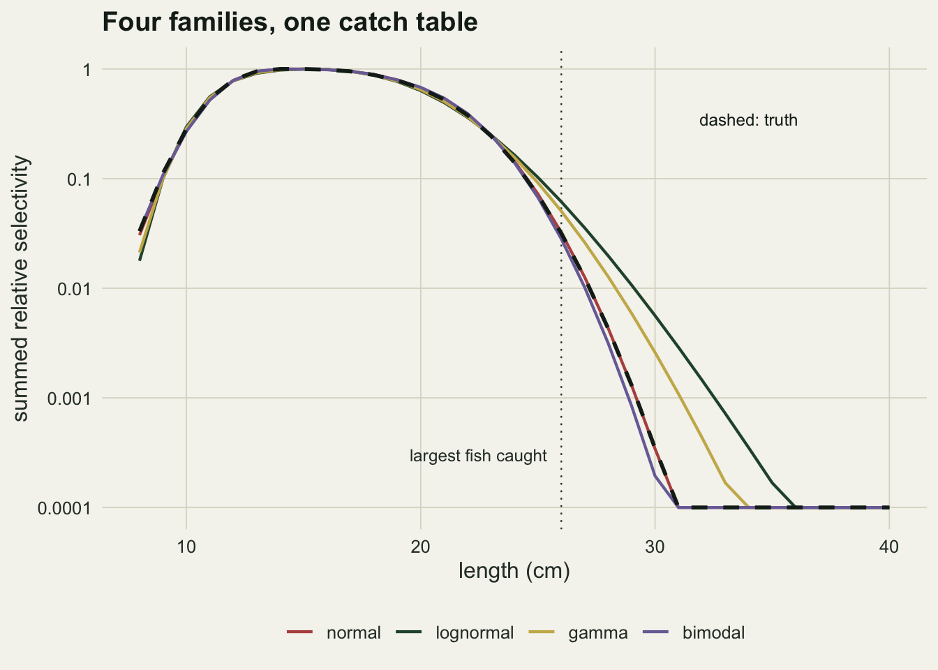
Inside the length range where fish were actually caught the five curves are hard to tell apart. Past the last fish they separate by orders of magnitude, and the divisor for the correction in exactly those classes is whichever number the chosen family happens to supply. In this replicate the fitted normal-scale and bi-normal curves happen to follow the truth closely and the lognormal and gamma curves run well above it, which means their divisors are larger and their corrected counts smaller.
The divisor is only half of the arithmetic, though, and in the blind zone it is the smaller half. Dividing by a small number does nothing to a numerator that is zero, and most of the blind-zone classes in a survey of this size have no fish in them at all.
set.seed(6208)
nonempty_big <- function(mesh, n_fish, reps = 3000) {
  lam <- f_pop * outer(len, mesh, fams[["normal"]], th = th_true[["normal"]])
  lam <- rowSums(lam / sum(lam) * n_fish)[is_big]
  draws <- matrix(rpois(reps * length(lam), rep(lam, times = reps)), ncol = reps)
  c(mean_classes = mean(colSums(draws > 0)), none = sum(colSums(draws) == 0), reps = reps)
}
ne3 <- nonempty_big(mesh_three, n_fish_std)
ne4 <- nonempty_big(mesh_four,  n_fish_std)
At three meshes and 800 fish, a survey has fish in 1.78 of the 16 length classes at or above the cut on average, and 118 of 3000 simulated surveys caught nothing at all above the cut. At four meshes the figure is 6.79 classes, and 0 of 3000 surveys came up empty there. Those are the numerators. The corrected distribution in the blind zone is a handful of ones and twos divided by a number close to zero, and both halves of that quotient are unstable in their own way: most classes contribute nothing whatever the family says, and the rare class that does contribute is multiplied by a very large factor that the family chose.
The right family does not give the large fish back
The grid below runs the whole thing: two mesh series, two truth families, three catch sizes, four fitted families, and 300 replicate surveys in every cell. Each replicate draws a fresh Poisson catch table, fits all four families to it, divides the pooled catch by each fitted summed selectivity, and records the corrected share of fish at or above the cut and the corrected mean length. The summary for each cell is the median over replicates and the interquartile range, with a bootstrap standard error on the median so the comparisons below are not read more finely than the replication supports.
n_rep  <- 300
cells  <- expand.grid(n_fish = c(300, 800, 3000), truth = c("normal", "bimodal"),
                      series = c("three", "four"), stringsAsFactors = FALSE)
cells  <- cells[!(cells$truth == "bimodal" & cells$n_fish != n_fish_std), ]
mesh_of <- list(three = mesh_three, four = mesh_four)

set.seed(9143)
runs <- lapply(seq_len(nrow(cells)), function(i)
  t(replicate(n_rep, one_survey(mesh_of[[cells$series[i]]], cells$truth[i],
                                cells$n_fish[i]))))
names(runs) <- paste(cells$series, cells$truth, cells$n_fish, sep = "_")

boot_se_median <- function(x, b = 400) {
  sd(replicate(b, median(sample(x, length(x), replace = TRUE))))
}
cell_stat <- function(key, column) {
  v <- runs[[key]][, column]
  c(med = median(v), iqr = IQR(v), se = boot_se_median(v))
}
right_fam <- c(normal = "normal", bimodal = "bimodal")

tab3n <- sapply(c("raw", names(fams)), function(fm)
  cell_stat("three_normal_800", if (fm == "raw") "raw_big" else paste0("big_", fm)))
tab3b <- sapply(c("raw", names(fams)), function(fm)
  cell_stat("three_bimodal_800", if (fm == "raw") "raw_big" else paste0("big_", fm)))
tab4n <- sapply(c("raw", names(fams)), function(fm)
  cell_stat("four_normal_800", if (fm == "raw") "raw_big" else paste0("big_", fm)))
tab4b <- sapply(c("raw", names(fams)), function(fm)
  cell_stat("four_bimodal_800", if (fm == "raw") "raw_big" else paste0("big_", fm)))

right3n <- tab3n["med", "normal"];  iqr3n <- tab3n["iqr", "normal"];  se3n <- tab3n["se", "normal"]
right3b <- tab3b["med", "bimodal"]; iqr3b <- tab3b["iqr", "bimodal"]; se3b <- tab3b["se", "bimodal"]
wrong3b <- range(tab3b["med", setdiff(names(fams), "bimodal")])
mean3n  <- cell_stat("three_normal_800", "mean_normal")
rawmean3n <- cell_stat("three_normal_800", "raw_mean")
big3n_all <- runs[["three_normal_800"]][, "big_normal"]
big3n_mean <- mean(big3n_all); big3n_max <- max(big3n_all)
share_below <- mean(runs[["three_normal_800"]][, "big_normal"] < truth_big)
share_se    <- sqrt(share_below * (1 - share_below) / n_rep)
Under the normal-scale truth and the three-mesh series the correctly specified correction returns a median large-fish share of 0.0522 (bootstrap standard error 0.0032) against the true 0.1109, with an interquartile range of 0.0765. The raw share was 0.0038, so the correction moves the estimate a long way in the right direction and still stops well short. Its spread is the other half of the problem: an interquartile range of 0.0765 is 0.69 times the quantity being estimated, so replicate surveys of the same lake, with the same gear and the same correction, disagree with each other over a range most of the size of the answer. 0.750 of replicates (standard error 0.025) land below the truth. The corrected mean length is 14.95 cm against a raw 14.76 cm and a true 15.75 cm, so the correction recovers 0.19 of the raw bias in the mean and leaves it 5 per cent low. It is still the easier target by a wide margin, and that is a statement about the starting point rather than about the correction: the raw mean is 6 per cent low where the raw large-fish share is 97 per cent low, because the mean is dominated by the length classes the gear does sample.
Two of the three rival families are genuinely misspecified under this truth, and both land below the correctly specified fit: the lognormal at 0.0317 and the gamma at 0.0372 against 0.0522. The third, the bi-normal, is not a misspecified rival at all when the truth is normal-scale: it contains that curve as a special case, with three spare parameters, for the reason set out in the next section, and it gives 0.0540. So choosing correctly between the families that could actually be wrong moves the median by 0.0149, against 0.0587 still missing once the right family has been chosen. The family decision is worth about a quarter of the shortfall it cannot touch, and that is the first half of the finding.
The median is not the whole story either. Over the same replicates the mean corrected share is 0.0895, much nearer the true 0.1109 than the median is, and the largest single replicate returns 0.94. The estimator is not badly off in expectation; it is the individual survey that cannot be used, because the mean is carried by the few replicates that happened to catch a fish in a class where the divisor is near zero, and a survey report carries one replicate.
The second half is what happens when the truth changes. Under the bi-normal truth the right family gives 0.1148 with an interquartile range of 0.0372, close to the true 0.1109, and the three wrong families give 0.1305 to 0.1587, above the truth instead of below it. The upper blind zone explains both cells: under the bi-normal truth the three-mesh series is blind only above 31 cm, so the fish the report is counting were caught rather than extrapolated, and every family does better. The sign of a family error is not a property of the family. It is a property of how the family’s tail compares with the tail of whatever is actually happening in the net, and a survey has no way to know that.
box_df <- do.call(rbind, lapply(c("normal", "bimodal"), function(tf) {
  mat <- runs[[paste0("three_", tf, "_", n_fish_std)]]
  do.call(rbind, lapply(names(fams), function(fm)
    data.frame(truth = tf, family = fm, value = mat[, paste0("big_", fm)])))
}))
box_df$family <- factor(box_df$family, levels = names(fams))
clip_hi   <- 0.32
clip_frac <- mean(box_df$value > clip_hi)
clip_max  <- max(box_df$value)
box_df$truth  <- factor(box_df$truth, levels = c("normal", "bimodal"),
                        labels = c("normal-scale truth", "bi-normal truth"))
raw_df <- data.frame(truth = factor(c("normal-scale truth", "bi-normal truth"),
                                    levels = levels(box_df$truth)),
                     value = c(tab3n["med", "raw"], tab3b["med", "raw"]))

ggplot(box_df, aes(family, value)) +
  geom_hline(yintercept = truth_big, linetype = "dashed",
             colour = te_ink, linewidth = 0.5) +
  geom_hline(data = raw_df, aes(yintercept = value), linetype = "dotted",
             colour = te_rust, linewidth = 0.6) +
  geom_boxplot(fill = te_gold, colour = te_ink, alpha = 0.45,
               outlier.size = 0.5, outlier.colour = te_body, linewidth = 0.35) +
  facet_wrap(~ truth) +
  coord_cartesian(ylim = c(0, clip_hi)) +
  labs(x = "fitted selectivity family", y = "corrected share at or above 25 cm",
       title = "Three meshes: corrected large-fish share by family",
       subtitle = "dashed: the truth; dotted: the raw catch share") +
  theme_datasheet() +
  theme(strip.text = element_text(colour = te_ink, face = "bold"))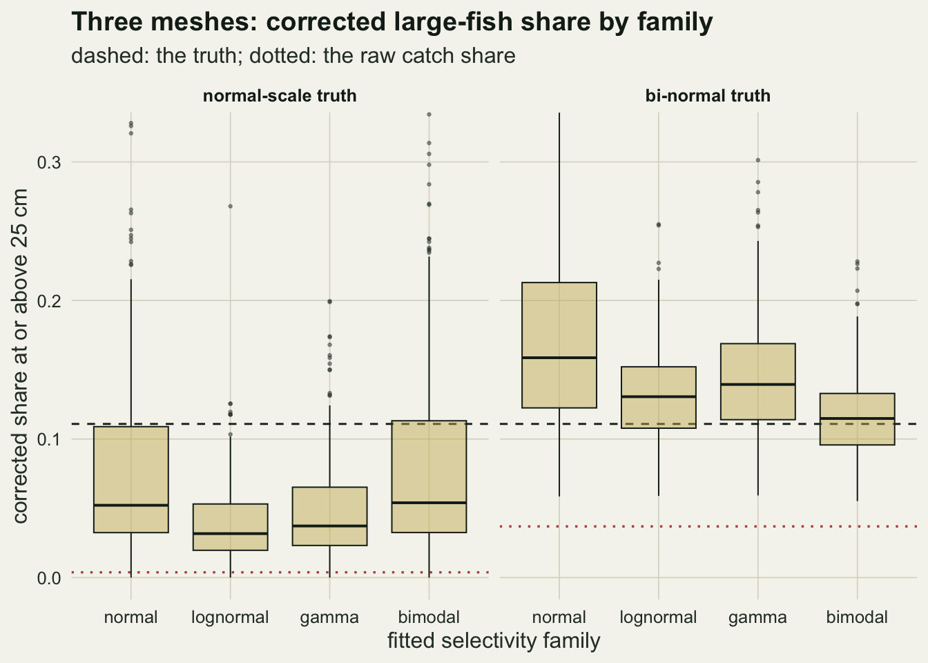
The panels are cut at 0.32: 1.9 per cent of the plotted replicates sit above the top, and the largest of them is 0.94, 8.5 times the truth. Those replicates are the mechanism rather than an exception to it. They are the surveys that found one fish in a class where the fitted selectivity is a thousandth of its peak, and the quotient then lands anywhere.
The fit statistic cannot settle it, and AIC only half can
The obvious response is to let the data choose the family. It cannot, for a reason that has nothing to do with gill nets: the bi-normal family contains the normal-scale family as the special case where the second component’s height goes to zero, so its maximised likelihood is never worse. An unpenalised deviance comparison over a set that contains a nesting pair is not a comparison at all.
pick_by <- function(key, stat) {
  mat <- runs[[key]][, paste0(stat, "_", names(fams))]
  factor(names(fams)[apply(mat, 1, which.min)], levels = names(fams))
}
dev3n <- table(pick_by("three_normal_800", "dev"))
aic3n <- table(pick_by("three_normal_800", "aic"))
dev3b <- table(pick_by("three_bimodal_800", "dev"))
aic3b <- table(pick_by("three_bimodal_800", "aic"))

aic_right_n <- as.numeric(aic3n["normal"]) / n_rep
aic_right_b <- as.numeric(aic3b["bimodal"]) / n_rep
aic_se_n    <- sqrt(aic_right_n * (1 - aic_right_n) / n_rep)
aic_se_b    <- sqrt(aic_right_b * (1 - aic_right_b) / n_rep)

sel_big <- function(key, stat) {
  mat <- runs[[key]]
  pk  <- as.character(pick_by(key, stat))
  mat[cbind(seq_len(nrow(mat)), match(paste0("big_", pk), colnames(mat)))]
}
aicsel3n <- sel_big("three_normal_800", "aic")
aicsel_med <- median(aicsel3n); aicsel_iqr <- IQR(aicsel3n)
aicsel_se  <- boot_se_median(aicsel3n)
Over the 300 replicates at three meshes under the normal-scale truth, the smallest deviance belonged to the bi-normal family in 299 of them and to the gamma family in 1; the normal-scale family, which generated the data, took it in 0. AIC, which charges the bi-normal three extra parameters, picks the normal-scale family in 0.780 of replicates (standard error 0.024); under the bi-normal truth it picks the bi-normal family in 0.937 (standard error 0.014). So AIC does recover the generating family most of the time, and it still does not help, because what it recovers is the family that fits the catch table, and the catch table is empty where the answer lives. Feeding the AIC-selected family into the correction gives a median large-fish share of 0.0519 (bootstrap standard error 0.0036) with an interquartile range of 0.0760: the same place the correctly specified fit landed, and no better.
This is the point checking a dispersal kernel makes about seeds and extrapolating a species-area curve beyond the plots about richness, arriving here in fishing gear. What is different is the advice that follows from it. There the recommendation is to report a quantity the data can support, a within-data quantile instead of a far-tail probability. A lake survey cannot take that advice, because the share of fish over the angling size is the product.
More fish does not fix it; another mesh does
scale_df <- do.call(rbind, lapply(c("three", "four"), function(sr)
  do.call(rbind, lapply(c(300, 800, 3000), function(nf) {
    st <- cell_stat(paste(sr, "normal", nf, sep = "_"), "big_normal")
    data.frame(series = sr, n_fish = nf, med = st["med"], iqr = st["iqr"], se = st["se"])
  }))))
scale_df$lo <- scale_df$med - scale_df$iqr / 2
scale_df$hi <- scale_df$med + scale_df$iqr / 2
scale_df$series <- factor(scale_df$series, levels = c("three", "four"),
                          labels = c("three meshes (20/25/31)", "four meshes (20/25/31/39)"))

ggplot(scale_df, aes(n_fish, med, colour = series)) +
  geom_hline(yintercept = truth_big, linetype = "dashed",
             colour = te_body, linewidth = 0.4) +
  geom_errorbar(aes(ymin = lo, ymax = hi), width = 0.06, linewidth = 0.5,
                position = position_dodge(width = 0.12)) +
  geom_point(size = 2.6, position = position_dodge(width = 0.12)) +
  scale_x_log10(breaks = c(300, 800, 3000)) +
  scale_colour_manual(values = c("three meshes (20/25/31)" = te_rust,
                                 "four meshes (20/25/31/39)" = te_gold)) +
  coord_cartesian(ylim = c(0, 0.22)) +
  labs(x = "fish measured per survey", y = "corrected share at or above 25 cm",
       colour = NULL, title = "Catch size does not close the gap") +
  theme_datasheet() + theme(legend.position = "bottom")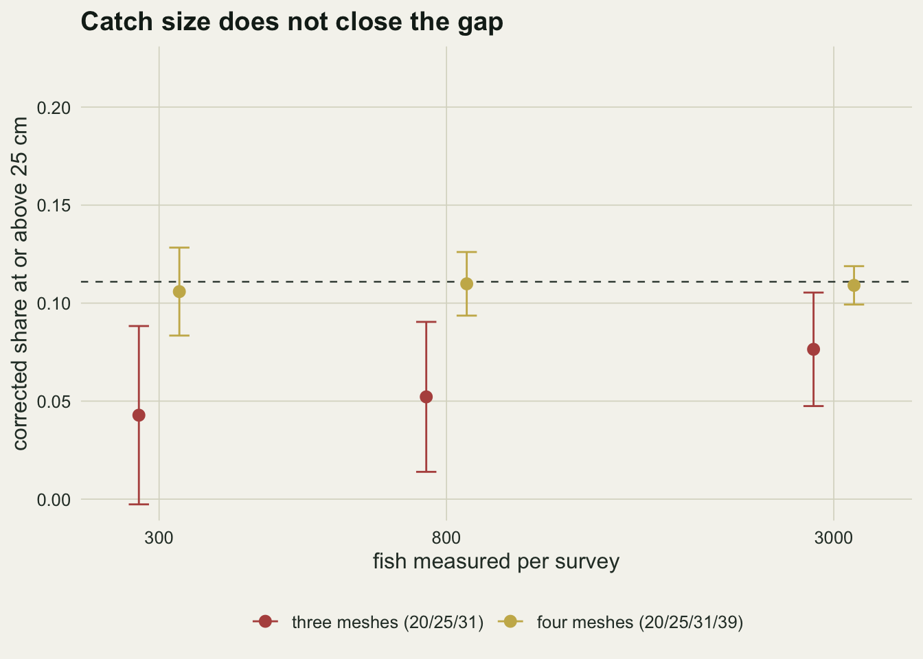
three_by_n <- sapply(c(300, 800, 3000), function(nf)
  cell_stat(paste("three", "normal", nf, sep = "_"), "big_normal"))
four_by_n  <- sapply(c(300, 800, 3000), function(nf)
  cell_stat(paste("four", "normal", nf, sep = "_"), "big_normal"))
colnames(three_by_n) <- colnames(four_by_n) <- c("300", "800", "3000")

four_all_n <- tab4n["med", names(fams)]
four_all_b <- tab4b["med", names(fams)]
four_worst <- max(abs(c(four_all_n, four_all_b) - truth_big))
four_iqr_n <- tab4n["iqr", names(fams)]
Raising the catch from 300 to 3000 fish moves the three-mesh median from 0.0428 to 0.0764, against the true 0.1109, while the interquartile range falls only from 0.0910 to 0.0579. Ten times the fieldwork closes part of the gap and leaves 0.0345 of it standing. The four-mesh series at the same three catch sizes gives 0.1059, 0.1098 and 0.1091, with the interquartile range falling from 0.0449 to 0.0196. The four-mesh series at 300 fish is closer to the truth, and tighter, than the three-mesh series at 3000: one extra panel is worth more than ten times the measuring.
The family dependence goes with it. At four meshes and 800 fish the four fitted families give 0.1098, 0.1083, 0.1078 and 0.1108 under the normal-scale truth and 0.1012, 0.1063, 0.1047 and 0.1092 under the bi-normal truth. The largest departure from the truth anywhere in that set is 0.0097. The families stop disagreeing because the extra mesh puts catch into the length classes where they used to disagree, and once there is data there, all four are estimating rather than extrapolating.
What to report
Publish the mesh series, not just the phrase multi-mesh. The three sizes used here and the four-mesh version differ in one panel and give different answers to the question the survey was run to answer. A reader cannot judge a corrected size structure without knowing the largest mesh in the series.
Give the length at which the fitted summed selectivity drops below a stated fraction of its peak, and the share of the corrected distribution that sits above that length. Those two numbers together say how much of the reported distribution is extrapolation. In this design at three meshes, with the threshold set at 10 per cent of peak, the upper blind zone begins at 25 cm and holds 0.1109 of the population under the normal-scale truth. Both numbers move with the threshold and with the largest mesh, which is exactly why the fraction has to be printed next to them, and no correction recovers that share in any one survey.
Report the raw catch share next to the corrected one. The gap between them is the size of the adjustment being asked for, and when the median corrected share is 14 times the raw one, as it is here at three meshes, that is information the reader should have.
Do not choose a selectivity family by unpenalised deviance when the candidate set contains a nesting pair. The bi-normal took the smallest deviance in 299 of 300 replicates generated from a normal-scale curve, which is what nesting does and not evidence of anything. AIC is the minimum fix; it recovers the generating family in 0.780 of replicates here and still leaves the corrected tail where it was.
Attach a replicate-level spread to any corrected tail quantity, from a simulation of the survey’s own gear and its own fitted curve. The interquartile range at three meshes and 800 fish is 0.0765 around a target of 0.1109; the same calculation at four meshes gives 0.0325. The code above is enough to produce it for a real series: put the fitted curve in as the truth and the observed catch size in as the effort.
If the large-fish share is the product, the repair is a panel of larger mesh, not a better model. That is the least welcome sentence in this post, because gear costs money and models are free, and it is the one the numbers support most clearly.
Honest limits
Only relative selectivity between meshes is identified here, and the simulation is built that way too: every panel is assumed to fish with the same power, and the population is assumed equally available to all of them. Real series set equal panel lengths partly for this reason, but fishing power can still differ between panels, and any difference goes straight into the fitted curve as if it were selectivity. Millar and Fryer discuss how a split or relative-power parameter enters when it can be estimated; nothing here estimates one.
The catch table is independent Poisson by length class and mesh. Real gill-net catches are clustered, because fish arrive in shoals and a net that has caught fish fishes differently from an empty one. Overdispersion would widen every interquartile range above; what it does to the medians is not measured here, and with a divisor near zero it cannot be assumed to leave them alone. Net saturation over a long soak would act like a length-dependent reduction in effort, which is a bias the conditional likelihood cannot see.
The truth is one fixed curve per run, with no variation between sets or nights. The trawl post on this site measures what between-haul variation in L50 does to an L50 interval, holding the selection range fixed across hauls, and the same question applies to a gill-net series; it is not asked here.
The blind-zone threshold of 10 per cent of peak summed selectivity is a convention, not a property of the gear. A lower threshold narrows the blind zone and shrinks the share of the reported distribution that gets flagged as extrapolation, without changing anything about what the gear caught; the point of the number is to force one explicit statement, not to be a standard.
Two truth families were used, normal-scale and bi-normal. The real curve need not be either, and the case where the fitted set contains nothing close to the truth is worse than anything measured here, not better. The families were fitted in the parametric form Millar and Fryer set out; the log-linear formulation of Millar and Holst also allows a non-parametric length effect, which would stabilise the division in the sparse classes. It would not create information beyond the last mesh, because the log-linear model estimates the length effect from the same empty cells.
The correction used is the simplest one: pooled catch divided by fitted summed selectivity, class by class. Where the divisor is near zero and the numerator is a small Poisson count, the quotient is unstable by construction, which is a large part of the interquartile ranges reported above. Truncating the corrected distribution at the last length with a usable divisor, or fitting numbers-at-length jointly with the selectivity parameters, would both behave better, and both would report less rather than recovering more.
Three and four panels are a short series. Survey nets in routine use carry many more panels over a wider mesh range, and the blind zone at both ends narrows accordingly; the arithmetic does not change, and neither does the question a report has to answer, which is where the largest panel’s mode sits relative to the length the managers asked about. The series here was kept short so that the blind zone is visible in a figure, and the four-mesh comparison is the smallest change that makes the point.
Everything here is one population with a fixed length distribution and a fixed cut at 25 cm. Move the cut down into the range the gear samples and the corrected estimate becomes reliable; move it up and it gets worse. The number that matters for a given survey is where the cut sits relative to the last mesh’s mode, and that is a property of the pairing, not of either one.
References
Millar RB, Holst R 1997 ICES Journal of Marine Science 54(3):471-477 (10.1006/jmsc.1996.0196)
Millar RB 1992 Journal of the American Statistical Association 87(420):962-968 (10.1080/01621459.1992.10476250)
Millar RB, Fryer RJ 1999 Reviews in Fish Biology and Fisheries 9(1):89-116 (10.1023/A:1008838220001)