Fishing, age truncation and spawning variability

Fishing old fish raises the CV of spawning output by a closed-form filter. In R: a 50-year survey index often misses it; the naive variance test is oversized.

A larval survey has sampled the same grid of stations off a coast for fifty years. Some of the species in the plankton are fished and some are not, and a plot of the yearly larval index shows the fished ones swinging harder from year to year. Hsieh and colleagues made that comparison on the California Cooperative Oceanic Fisheries Investigations series in 2006 and found the exploited species more variable; Anderson and colleagues returned to the question in 2008 and found little support for truncated stocks simply tracking the environment more closely, and strong support for less stable dynamics driven by higher intrinsic growth rates. The averaging picture they weighed and largely set aside is still the one usually drawn: a stock with many age classes averages over many recruitment years, and a stock reduced to a few young age classes cannot. This post quantifies that linear part, and the Beverton-Holt feedback below is the nearest this model comes to their third mechanism.

That picture can be written as a formula, and the formula is short enough that it should come first rather than last. This post derives it, checks the code against it to machine precision, and then spends its effort on the questions the formula leaves open: how much the stock-recruitment feedback adds, what fishing does to the spectrum of spawning output, and whether a fifty year index with ordinary observation error can see the change at all.

The positioning against the neighbouring posts is narrow. Stock-recruitment and reference points computes spawning potential ratio (SPR) targets and equilibrium yield, and everything in it is an equilibrium: its section on what a per-recruit target buys says nothing about variance. Here the same Beverton-Holt steepness form and the same SPR scale are used, and the question is the variability around that equilibrium. Red noise and extinction risk in a Ricker model treats environmental noise in an unstructured population and says in its honest limits that the stage structured comparison is not made; this post is an age structured model with white recruitment noise, so it covers the other half. Spectral analysis of population cycles supplies the smoothed periodogram and the warning that a red spectrum is not a cycle, which is the reading used below. Early warning signals and critical slowing already shows variance rising as a system nears a fold; the rise near the crash point here is the same mechanism and is cited, not sold again. The age classes and survivorship are those of a Leslie matrix model, which is the prerequisite.

library(ggplot2)

te_paper  <- "#f5f4ee"
te_ink    <- "#16241d"
te_body   <- "#2c3a31"
te_forest <- "#275139"
te_rust   <- "#b5534e"
te_gold   <- "#c9b458"
te_line   <- "#dad9ca"

theme_datasheet <- function() {
  theme_minimal(base_size = 12) +
    theme(plot.background  = element_rect(fill = te_paper, colour = NA),
          panel.background = element_rect(fill = te_paper, colour = NA),
          panel.grid.major = element_line(colour = te_line, linewidth = 0.3),
          panel.grid.minor = element_blank(),
          text             = element_text(colour = te_body),
          plot.title       = element_text(colour = te_ink, face = "bold"),
          plot.subtitle    = element_text(colour = te_body),
          axis.text        = element_text(colour = te_body))
}

Spawning output is a weighted sum of past recruitments

The stock has 25 age classes with a plus group, natural mortality of 0.2 per year, fecundity proportional to a von Bertalanffy weight and zero below the age at maturity of 5 years. Recruitment follows the Beverton-Holt curve in steepness form on spawning output, with steepness fixed at 0.7, and each year’s recruitment is multiplied by an independent lognormal deviation with log scale standard deviation 0.5 and mean one. Fishing is expressed only through the SPR it produces, never as a raw fishing mortality, because the same SPR needs very different mortality rates under different selectivities. All of these constants were fixed before anything ran.

n_age   <- 25
m_nat   <- 0.2
sd_rec  <- 0.5
cv_rec  <- sqrt(exp(sd_rec^2) - 1)
lag_max <- 600

make_stock <- function(age_mat = 5, h_steep = 0.7) {
  ages <- seq_len(n_age)
  fec  <- (1 - exp(-0.25 * ages))^3 * (ages >= age_mat)
  stk  <- list(ages = ages, fec = fec, mature = as.numeric(ages >= age_mat),
               h = h_steep, age_mat = age_mat)
  stk$e0 <- eggs_per_recruit(stk, rep(0, n_age))
  stk
}

surv_to_age <- function(f_vec) {
  z_vec <- m_nat + f_vec
  c(1, exp(-cumsum(z_vec[-n_age])))
}

eggs_per_recruit <- function(stk, f_vec, fec_mult = 1) {
  z_vec <- m_nat + f_vec
  l_vec <- surv_to_age(f_vec)
  l_vec[n_age] <- l_vec[n_age] / (1 - exp(-z_vec[n_age]))
  sum(l_vec * stk$fec * fec_mult)
}

spr_of <- function(stk, f_vec, fec_mult = 1) {
  eggs_per_recruit(stk, f_vec, fec_mult) / stk$e0
}

f_for_spr <- function(stk, spr, sel) {
  if (spr == 1) return(0)
  uniroot(function(f_val) spr_of(stk, f_val * sel) - spr,
          c(0, 10), tol = 1e-12)$root
}

lag_weights <- function(stk, f_vec, fec_mult = 1) {
  z_vec <- m_nat + f_vec
  l_vec <- surv_to_age(f_vec)
  lags  <- seq_len(lag_max)
  w_vec <- numeric(lag_max)
  young <- seq_len(n_age - 1)
  w_vec[young] <- stk$fec[young] * l_vec[young]
  old <- n_age:lag_max
  w_vec[old] <- stk$fec[n_age] * l_vec[n_age] * exp(-z_vec[n_age] * (old - n_age))
  w_vec * fec_mult
}

base_stock <- make_stock()
h_base     <- base_stock$h
spr_crash  <- (1 - h_base) / (4 * h_base)
spr_grid   <- c(1, 0.6, 0.45, 0.3, 0.2, 0.15)
f_mature   <- vapply(spr_grid, function(s) f_for_spr(base_stock, s, base_stock$mature), 0)
f_all      <- vapply(spr_grid, function(s) f_for_spr(base_stock, s, rep(1, n_age)), 0)
row_30     <- which(spr_grid == 0.3)
row_15     <- which(spr_grid == 0.15)

The population cannot persist below an SPR of 0.1071, which for Beverton-Holt recruitment is one minus steepness over four times steepness. The SPR grid runs from unfished down to 0.15, and an SPR of 0.3 needs a fishing mortality of 0.386 per year when only mature fish are taken, but only 0.144 when every age from one upwards is fished.

The formula follows from bookkeeping. A fish of age a in year t recruited in year t minus a and has survived to age a with probability l(a). Spawning output in year t is therefore a sum over lags, E(t) = sum over a of w(a) R(t minus a), with weight w(a) equal to fecundity at age a times survival to age a; the plus group contributes a geometric tail of further lags with ratio exp(minus Z) at the oldest age. When recruitments are independent with mean mu and standard deviation sigma, and the stock-recruitment feedback is switched off, the mean of E is mu times the sum of weights and its variance is sigma squared times the sum of squared weights. So

CV(E) = CV(R) sqrt(sum w^2) / sum w = CV(R) / sqrt(n_c),

where n_c = (sum w)^2 / sum w^2 is the effective number of cohorts contributing to spawning. Fishing mature fish removes weight from the old lags and lowers n_c. Cutting fecundity by a constant factor multiplies every weight by the same number, leaves n_c unchanged, and so leaves the CV exactly where it was: that control is depletion without truncation, at the same SPR. Fishing every age at a lower rate reaches the same SPR partly by killing fish before they mature, so it truncates the mature age structure less.

run_stock <- function(stk, f_mat, fec_mult, feedback, eps, burn) {
  n_col  <- ncol(f_mat)
  n_step <- if (is.matrix(eps)) nrow(eps) else length(eps)
  z_mat  <- m_nat + f_mat
  s_mat  <- exp(-z_mat)
  h_s    <- stk$h
  spr_c  <- vapply(seq_len(n_col), function(k) spr_of(stk, f_mat[, k], fec_mult[k]), 0)
  r_eq   <- (4 * h_s * spr_c - (1 - h_s)) / ((5 * h_s - 1) * spr_c)
  n_mat  <- vapply(seq_len(n_col), function(k) {
    l_vec <- surv_to_age(f_mat[, k])
    l_vec[n_age] <- l_vec[n_age] / (1 - exp(-z_mat[n_age, k]))
    l_vec * r_eq[k]
  }, numeric(n_age))
  fec_mat <- stk$fec %o% fec_mult
  out <- matrix(0, n_step - burn, n_col)
  for (i in seq_len(n_step)) {
    e_now <- colSums(n_mat * fec_mat)
    if (i > burn) out[i - burn, ] <- e_now
    dev_i <- if (is.matrix(eps)) exp(eps[i, ]) else exp(eps[i])
    r_bh  <- 4 * h_s * e_now / (stk$e0 * (1 - h_s) + (5 * h_s - 1) * e_now)
    r_new <- ifelse(feedback, r_bh, r_eq) * dev_i
    plus  <- n_mat[n_age, ] * s_mat[n_age, ]
    n_mat[2:n_age, ] <- n_mat[1:(n_age - 1), ] * s_mat[1:(n_age - 1), ]
    n_mat[n_age, ]   <- n_mat[n_age, ] + plus
    n_mat[1, ]       <- r_new
  }
  list(e_out = out, r_eq = r_eq)
}

long_len  <- 20000
long_burn <- 700
set.seed(4417)
eps_long <- rnorm(long_len + long_burn, -sd_rec^2 / 2, sd_rec)

n_spr   <- length(spr_grid)
scen    <- expand.grid(spr_i = seq_len(n_spr),
                       kind = c("mature", "all ages", "fecundity cut"),
                       feedback = c(FALSE, TRUE), stringsAsFactors = FALSE)
f_cols  <- vapply(seq_len(nrow(scen)), function(k) {
  i_s <- scen$spr_i[k]
  switch(scen$kind[k],
         "mature"        = f_mature[i_s] * base_stock$mature,
         "all ages"      = rep(f_all[i_s], n_age),
         "fecundity cut" = rep(0, n_age))
}, numeric(n_age))
fm_cols <- ifelse(scen$kind == "fecundity cut", spr_grid[scen$spr_i], 1)

t_long   <- system.time(
  long_run <- run_stock(base_stock, f_cols, fm_cols, scen$feedback, eps_long, long_burn)
)[["elapsed"]]

rec_long <- exp(eps_long)
id_err <- vapply(which(!scen$feedback), function(k) {
  w_k    <- lag_weights(base_stock, f_cols[, k], fm_cols[k])
  r_ser  <- long_run$r_eq[k] * rec_long
  e_filt <- stats::filter(r_ser, c(0, w_k), sides = 1)
  e_filt <- as.numeric(e_filt)[(long_burn + 1):(long_len + long_burn)]
  max(abs(e_filt - long_run$e_out[, k]) / long_run$e_out[, k])
}, 0)
id_max <- max(id_err)

cv_of <- function(x) sd(x) / mean(x)
n_block <- 10
block_id <- rep(seq_len(n_block), each = long_len / n_block)
scen$cv_sim <- apply(long_run$e_out, 2, cv_of)
scen$cv_se  <- apply(long_run$e_out, 2, function(x)
  sd(tapply(x, block_id, cv_of)) / sqrt(n_block))
scen$cv_formula <- vapply(seq_len(nrow(scen)), function(k) {
  w_k <- lag_weights(base_stock, f_cols[, k], fm_cols[k])
  cv_rec * sqrt(sum(w_k^2)) / sum(w_k)
}, 0)
scen$n_cohort <- vapply(seq_len(nrow(scen)), function(k) {
  w_k <- lag_weights(base_stock, f_cols[, k], fm_cols[k])
  sum(w_k)^2 / sum(w_k^2)
}, 0)
scen$gen_time <- vapply(seq_len(nrow(scen)), function(k) {
  w_k <- lag_weights(base_stock, f_cols[, k], fm_cols[k])
  sum(seq_len(lag_max) * w_k) / sum(w_k)
}, 0)

pick <- function(i_s, kind, fb) which(scen$spr_i == i_s & scen$kind == kind & scen$feedback == fb)
nofb_rows <- which(!scen$feedback)
z_gap     <- abs(scen$cv_sim[nofb_rows] - scen$cv_formula[nofb_rows]) / scen$cv_se[nofb_rows]
z_gap_max <- max(z_gap)
gap_max   <- max(abs(scen$cv_sim[nofb_rows] - scen$cv_formula[nofb_rows]))

cv_un   <- scen$cv_formula[pick(1, "mature", FALSE)]
cv_m30  <- scen$cv_formula[pick(row_30, "mature", FALSE)]
cv_a30  <- scen$cv_formula[pick(row_30, "all ages", FALSE)]
cv_c30  <- scen$cv_formula[pick(row_30, "fecundity cut", FALSE)]
nc_un   <- scen$n_cohort[pick(1, "mature", FALSE)]
nc_m30  <- scen$n_cohort[pick(row_30, "mature", FALSE)]
nc_a30  <- scen$n_cohort[pick(row_30, "all ages", FALSE)]
gt_un   <- scen$gen_time[pick(1, "mature", FALSE)]
gt_m30  <- scen$gen_time[pick(row_30, "mature", FALSE)]
gt_a30  <- scen$gen_time[pick(row_30, "all ages", FALSE)]

The check has two levels. The first is an identity, not a statistic: applying the weights directly to the recruitment series that drove the no-feedback simulations reproduces the simulated spawning output with a largest relative error of 3.68e-15 across all 18 no-feedback runs of 20000 years. The simulator and the formula are the same object. The second level is the CV itself, which the simulation only estimates. Across those runs the largest gap between simulated CV and formula is 0.0022, at most 0.7 block standard errors (ten blocks of 2000 years), so the third decimal of a simulated CV is Monte Carlo noise and the formula is the number to quote.

Unfished, the formula gives a CV of spawning output of 0.144 from a recruitment CV of 0.533, because 13.7 effective cohorts share the load. At an SPR of 0.3 with mature-only fishing the effective number falls to 4.6 and the CV rises to 0.247. Fishing all ages to the same SPR leaves 8.1 effective cohorts and a CV of 0.187, and the mean age of spawning output tells the same story: 10.9 years unfished, 6.7 under mature-only fishing and 8.3 under all-ages fishing. The fecundity cut gives 0.144, identical to unfished. Without feedback, depletion on its own does nothing to the CV.

w_show <- 20
w_df <- do.call(rbind, lapply(list(
  list(k = pick(1, "mature", FALSE), lab = "unfished"),
  list(k = pick(row_30, "mature", FALSE), lab = "SPR 0.3, mature ages fished"),
  list(k = pick(row_30, "all ages", FALSE), lab = "SPR 0.3, all ages fished"),
  list(k = pick(row_30, "fecundity cut", FALSE), lab = "SPR 0.3, fecundity cut")), function(el) {
    w_k <- lag_weights(base_stock, f_cols[, el$k], fm_cols[el$k])
    data.frame(age = seq_len(w_show), share = (w_k / sum(w_k))[seq_len(w_show)],
               case = el$lab)
  }))
w_df$case <- factor(w_df$case, levels = unique(w_df$case))

ggplot(w_df, aes(age, share, colour = case, linetype = case)) +
  geom_line(linewidth = 0.9) +
  geom_point(size = 1.6) +
  scale_colour_manual(values = c(te_ink, te_rust, te_gold, te_forest), name = NULL) +
  scale_linetype_manual(values = c("solid", "solid", "solid", "dashed"), name = NULL) +
  labs(x = "age (years)", y = "share of spawning output",
       title = "Fishing moves spawning onto the youngest mature ages",
       subtitle = "the fecundity cut has the unfished shape exactly (dashed)") +
  guides(colour = guide_legend(nrow = 2), linetype = guide_legend(nrow = 2)) +
  theme_datasheet() +
  theme(legend.position = "bottom")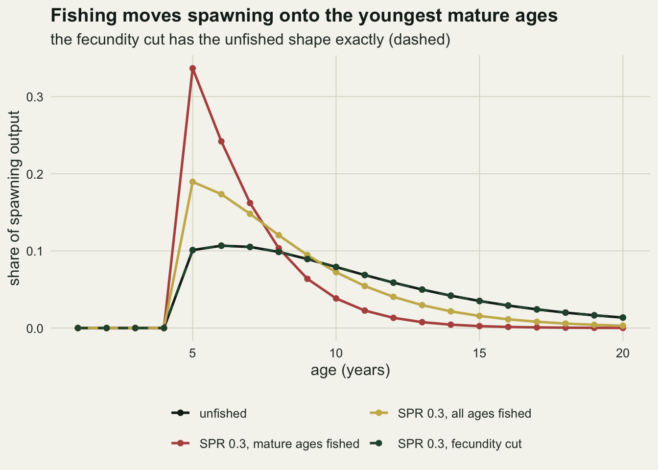

Figure 1: Share of spawning output contributed by each age, unfished and at an SPR of 0.3 under three ways of reaching it.

The feedback is an elasticity, and it is small until the crash

With the Beverton-Holt curve switched on, a year of high spawning output raises the next recruitment and a low one lowers it. Linearised on the log scale around the fished equilibrium, the recruitment response to a proportional change in spawning output is the elasticity beta = E0 (1 minus h) / (E0 (1 minus h) + (5h minus 1) E), and substituting the equilibrium spawning output gives the tidy result beta = SPR_crash / SPR. The elasticity is 0.107 unfished and reaches one at the crash point. The linearised process then has transfer function W(f) / (1 minus beta W(f)) with W the normalised weights, and its variance is the integral of the squared modulus over frequency. With beta at zero the integral returns the filter formula, which is a check on the numerical integration.

n_freq  <- 4000
freq_mid <- (seq_len(n_freq) - 0.5) / (2 * n_freq)
lag_seq  <- seq_len(lag_max)
transfer <- function(w_vec, freqs) {
  w_n <- w_vec / sum(w_vec)
  as.vector(exp(-2i * pi * outer(freqs, lag_seq)) %*% w_n)
}
lin_cv <- function(w_vec, beta) {
  w_f <- transfer(w_vec, freq_mid)
  cv_rec * sqrt(mean(Mod(w_f / (1 - beta * w_f))^2))
}

scen$beta   <- ifelse(scen$feedback, spr_crash / spr_grid[scen$spr_i], 0)
scen$cv_lin <- vapply(seq_len(nrow(scen)), function(k) {
  lin_cv(lag_weights(base_stock, f_cols[, k], fm_cols[k]), scen$beta[k])
}, 0)

parseval_gap <- max(abs(scen$cv_lin[nofb_rows] - scen$cv_formula[nofb_rows]))

fb_tab <- data.frame(spr = spr_grid,
  beta    = spr_crash / spr_grid,
  nofb    = scen$cv_formula[scen$kind == "mature" & !scen$feedback],
  fb_sim  = scen$cv_sim[scen$kind == "mature" & scen$feedback],
  fb_se   = scen$cv_se[scen$kind == "mature" & scen$feedback],
  fb_lin  = scen$cv_lin[scen$kind == "mature" & scen$feedback],
  cut_sim = scen$cv_sim[scen$kind == "fecundity cut" & scen$feedback],
  cut_lin = scen$cv_lin[scen$kind == "fecundity cut" & scen$feedback])
fb_tab$gain_sim <- fb_tab$fb_sim / fb_tab$nofb - 1
fb_tab$gain_lin <- fb_tab$fb_lin / fb_tab$nofb - 1
fb_tab$lin_err  <- fb_tab$fb_sim / fb_tab$fb_lin - 1
lin_err_mid <- max(abs(fb_tab$lin_err[fb_tab$spr >= 0.3]))

The integral agrees with the filter formula to 2.50e-16 when beta is zero. With the feedback on and mature-only fishing, the simulated CV exceeds the no-feedback formula by 1.2 per cent unfished, 5.7 per cent at an SPR of 0.3 and 29.8 per cent at 0.15, where beta is 0.71. So the filter alone explains the rise at ordinary target SPRs, and the feedback adds a correction of at most 5.7 per cent down to an SPR of 0.3.

The linearised feedback formula does most of the rest. Down to an SPR of 0.3 it matches the simulated CV to within 1.9 per cent; at 0.15 it gives 0.477 against a simulated 0.494 (block standard error 0.009), so the linearisation starts to fall short only close to the crash, where the curvature of the recruitment curve matters for deviations this large. The fecundity cut is no longer inert once feedback is on: its simulated CV is 0.161 at an SPR of 0.3 (formula 0.165) and 0.222 at 0.15. Depletion does raise variability, but only through the elasticity, and at target SPRs the amount is small next to the effect of removing old fish.

cv_df <- scen
cv_df$spr <- spr_grid[cv_df$spr_i]
cv_df$model <- ifelse(cv_df$feedback, "with feedback", "no feedback")

ggplot(cv_df, aes(spr, colour = kind)) +
  geom_vline(xintercept = spr_crash, linetype = "dotted", colour = te_body, linewidth = 0.6) +
  geom_line(aes(y = cv_lin), linewidth = 0.8) +
  geom_point(aes(y = cv_sim), size = 2.2) +
  facet_wrap(~ model) +
  scale_x_reverse(breaks = c(1, 0.6, 0.45, 0.3, 0.2, 0.15)) +
  scale_colour_manual(values = c("all ages" = te_gold, "fecundity cut" = te_forest,
                                 "mature" = te_rust), name = NULL) +
  labs(x = "spawning potential ratio (fishing increases to the right)",
       y = "CV of spawning output",
       title = "Truncation carries the rise; feedback adds to it near the crash",
       subtitle = "dotted line: crash SPR for steepness 0.7") +
  theme_datasheet() +
  theme(legend.position = "bottom")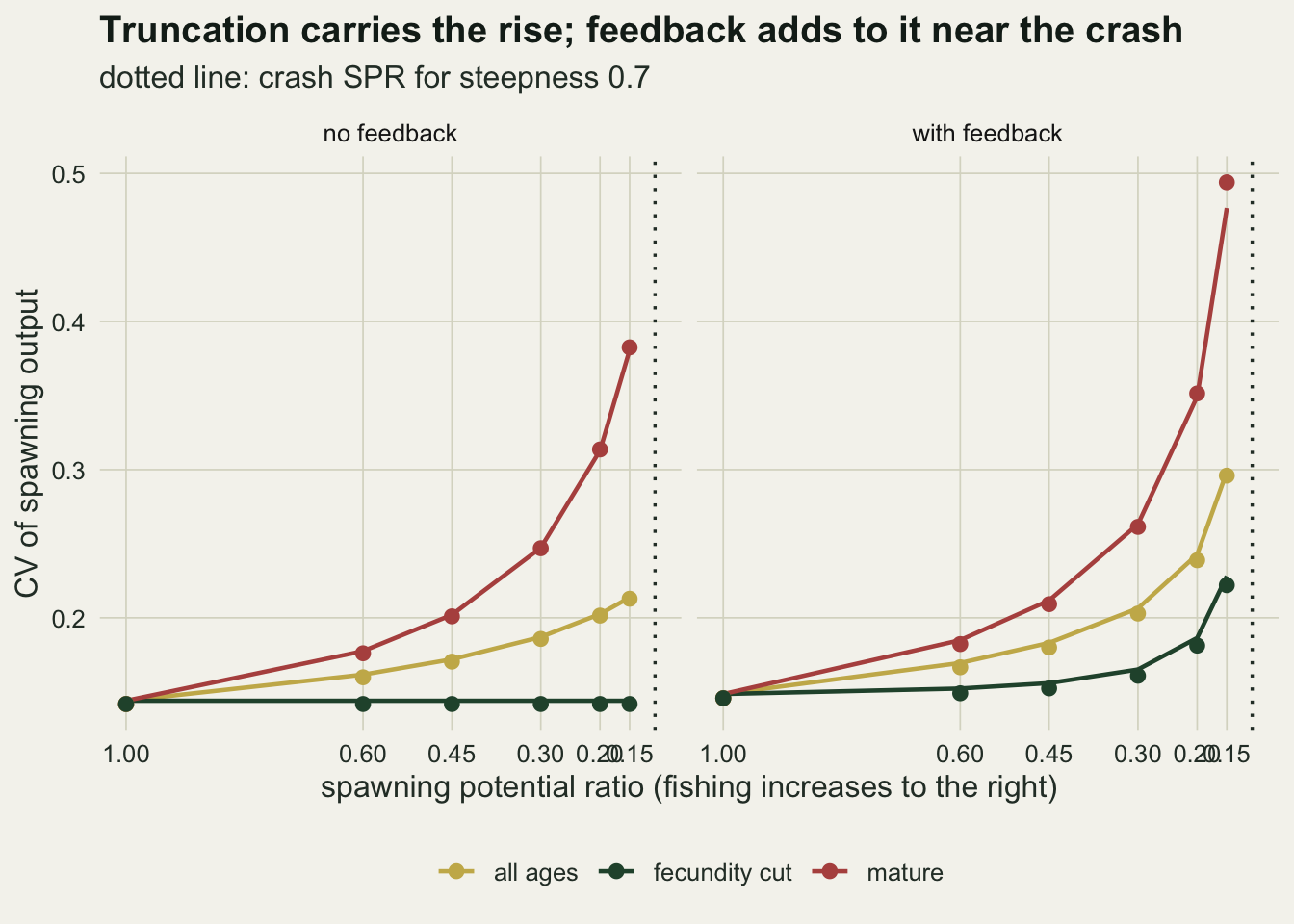

Figure 2: CV of spawning output against SPR. Lines are closed forms (filter without feedback, linearised feedback); points are 20000-year simulations.

Truncation whitens the spectrum; feedback can add a bump

The same transfer function says where in frequency the extra variance goes. The spectrum of spawning output is proportional to the squared modulus of W(f) / (1 minus beta W(f)). Because every weight is positive, the modulus of W at any frequency is at most its value at zero, and |1 minus beta W(f)| is at least 1 minus beta W(0), so the spectrum has its highest value at the lowest frequency, with or without feedback. That does not rule out a secondary local peak. Without feedback the filter is low-pass; with feedback, the denominator is smallest where the phase of W(f) returns to zero, which for weights concentrated on a few ages happens near one over the generation time, and a bump can appear there. Bjornstad, Nisbet and Fromentin used the name cohort resonance for the way age structure concentrates white recruitment noise into slow, trend-like fluctuations, and Worden, Botsford, Hastings and Holland described the sensitivity near the mean age of reproduction; the bump is that second part of the story. The check below computes both versions of the closed form, finds their local maxima on a grid of frequencies, and compares them with the smoothed periodogram of the long runs, spans c(51, 51) as fixed in advance.

spec_rows <- c(pick(1, "mature", FALSE), pick(row_30, "mature", FALSE),
               pick(1, "mature", TRUE), pick(row_30, "mature", TRUE),
               pick(row_15, "mature", TRUE))
spec_lab  <- c("unfished", "SPR 0.3, mature ages fished",
               "unfished", "SPR 0.3, mature ages fished",
               "SPR 0.15, mature ages fished")
low_cut   <- 1 / 8
spec_df <- do.call(rbind, lapply(seq_along(spec_rows), function(j) {
  k   <- spec_rows[j]
  s_p <- spec.pgram(long_run$e_out[, k], spans = c(51, 51), taper = 0,
                    detrend = FALSE, plot = FALSE)
  w_k <- lag_weights(base_stock, f_cols[, k], fm_cols[k])
  w_f <- transfer(w_k, s_p$freq)
  s_c <- Mod(w_f / (1 - scen$beta[k] * w_f))^2
  data.frame(freq = s_p$freq, periodogram = s_p$spec / mean(s_p$spec),
             closed = s_c / mean(s_c), case = spec_lab[j],
             model = ifelse(scen$feedback[k], "with feedback", "no feedback"))
}))

low_share <- function(case_lab, mod_lab, col) {
  d_c <- spec_df[spec_df$case == case_lab & spec_df$model == mod_lab, ]
  sum(d_c[[col]][d_c$freq < low_cut]) / sum(d_c[[col]])
}
low_un_c  <- low_share(spec_lab[1], "no feedback", "closed")
low_un_p  <- low_share(spec_lab[1], "no feedback", "periodogram")
low_30_c  <- low_share(spec_lab[2], "no feedback", "closed")
low_30_p  <- low_share(spec_lab[2], "no feedback", "periodogram")
low_un_fb <- low_share(spec_lab[1], "with feedback", "closed")
low_30_fb <- low_share(spec_lab[2], "with feedback", "closed")
low_15_fb <- low_share(spec_lab[5], "with feedback", "closed")

nofb_un <- spec_df[spec_df$case == spec_lab[1] & spec_df$model == "no feedback", ]
nofb_30 <- spec_df[spec_df$case == spec_lab[2] & spec_df$model == "no feedback", ]
ratio_spec  <- nofb_30$closed / nofb_un$closed
ratio_low   <- ratio_spec[1]
ratio_high  <- ratio_spec[length(ratio_spec)]
ratio_cross <- nofb_un$freq[which(ratio_spec > 1)[1]]

# local maxima of the closed-form spectrum on a regular frequency grid
freq_pk <- seq(0.0005, 0.5, by = 0.0005)
local_peaks <- function(w_vec, beta) {
  w_f <- transfer(w_vec, freq_pk)
  s_c <- Mod(w_f / (1 - beta * w_f))^2
  i_p <- which(diff(sign(diff(s_c))) == -2) + 1
  data.frame(freq = freq_pk[i_p], rel_low = s_c[i_p] / s_c[1],
             rel_trough = vapply(i_p, function(i) s_c[i] / min(s_c[seq_len(i)]), 0))
}
pk_nofb <- vapply(which(scen$kind == "mature" & !scen$feedback), function(k)
  nrow(local_peaks(lag_weights(base_stock, f_cols[, k], fm_cols[k]), 0)), 0)
pk_fb30 <- local_peaks(lag_weights(base_stock, f_cols[, pick(row_30, "mature", TRUE)], 1),
                       spr_crash / 0.3)
pk_fb15 <- local_peaks(lag_weights(base_stock, f_cols[, pick(row_15, "mature", TRUE)], 1),
                       spr_crash / 0.15)
gt_m15  <- scen$gen_time[pick(row_15, "mature", TRUE)]

# the same check for the maturity-at-8 stock used in the sensitivity runs
stk_8   <- make_stock(8, 0.7)
w_830   <- lag_weights(stk_8, f_for_spr(stk_8, 0.3, stk_8$mature) * stk_8$mature)
gt_830  <- sum(seq_len(lag_max) * w_830) / sum(w_830)
pk_830  <- local_peaks(w_830, spr_crash / 0.3)
pk_830n <- nrow(local_peaks(w_830, 0))

# the bump in the simulated periodogram, SPR 0.15 with feedback
pg_15  <- spec_df[spec_df$case == spec_lab[5], ]
pk_win <- abs(pg_15$freq - pk_fb15$freq[1]) < 0.05
pg_pk  <- which(pk_win)[which.max(pg_15$periodogram[pk_win])]
pg_tr  <- which(pg_15$freq > 0.05 & pg_15$freq < pg_15$freq[pg_pk])
pg_pk_freq  <- pg_15$freq[pg_pk]
pg_pk_ratio <- pg_15$periodogram[pg_pk] / min(pg_15$periodogram[pg_tr])

Without feedback, the closed form for mature-only fishing has no local maximum at any SPR on the grid (largest count 0): the spectrum falls from the lowest frequency to one half. Unfished, 0.945 of the variance of spawning output lies at frequencies slower than one cycle in eight years according to the closed form, and 0.942 according to the smoothed periodogram. At an SPR of 0.3 with mature-only fishing the shares are 0.727 and 0.720. Relative to its own mean level, the fished spectrum is 0.34 times the unfished one at the lowest frequency, crosses above it at 0.043 cycles per year, and is 5.49 times it at the Nyquist frequency of one half.

With feedback, the low-frequency shares from the closed form are 0.948 unfished, 0.738 at an SPR of 0.3 and 0.488 at 0.15. At an SPR of 0.3 the only local maximum is at 0.367 cycles per year, 0.021 of the value at the lowest frequency and 1.03 times the trough before it, which is a ripple and nowhere near one over the mean age of spawning output (0.149). At 0.15, where beta is 0.71, a clear bump sits at 0.187 cycles per year against one over the mean age of 0.183; its height is 0.19 of the value at the lowest frequency and 7.9 times the trough before it, with a smaller echo at 0.393, about twice that frequency. The simulated periodogram shows the same bump, with its highest point near there at 0.192 and 9.0 times its own trough. For the stock that matures at age 8, the one used in the sensitivity runs below, the weights are more concentrated and the bump appears already at an SPR of 0.3: at 0.1095 cycles per year against one over the mean age of 0.1105, 0.36 of the lowest-frequency value (without feedback that stock has none: count 0).

So in this model truncation on its own whitens the output: the low-frequency concentration that Bjornstad and colleagues called cohort resonance is weaker in the truncated stock, relative to its total variance. Worden and colleagues found that lower adult survival strengthens the response at all frequencies in absolute terms, which is not contradicted here, because the CV rises at the same time as the share moves. The feedback barely moves the low-frequency shares unfished and at an SPR of 0.3 (compare the two sets of shares above), and adds a second effect that grows with beta: a bump near one over the generation time once the weights sit on few ages. The bump is a property of the transfer function, driven by white noise, not an independent cycle.

thin_df <- spec_df[seq(1, nrow(spec_df), by = 40), ]
vl_df <- data.frame(model = c("no feedback", "no feedback", "with feedback", "with feedback", "with feedback"),
                    case = spec_lab,
                    x0 = 1 / c(gt_un, gt_m30, gt_un, gt_m30, gt_m15))
spec_cols <- c("unfished" = te_ink, "SPR 0.3, mature ages fished" = te_rust,
               "SPR 0.15, mature ages fished" = te_gold)
spec_df$case <- factor(spec_df$case, levels = names(spec_cols))
thin_df$case <- factor(thin_df$case, levels = names(spec_cols))
vl_df$case   <- factor(vl_df$case, levels = names(spec_cols))
ggplot(spec_df, aes(freq, closed, colour = case)) +
  geom_vline(data = vl_df, aes(xintercept = x0, colour = case),
             linetype = "dotted", linewidth = 0.6, show.legend = FALSE) +
  geom_point(data = thin_df, aes(y = periodogram), size = 1.1, alpha = 0.6) +
  geom_line(linewidth = 0.9) +
  facet_wrap(~ model, ncol = 1) +
  scale_y_log10() +
  scale_colour_manual(values = spec_cols, name = NULL) +
  labs(x = "frequency (cycles per year)", y = "spectrum relative to its mean (log scale)",
       title = "Fishing flattens the spectrum; feedback adds a bump",
       subtitle = "dotted lines: one over the mean age of spawning output") +
  theme_datasheet() +
  theme(legend.position = "bottom")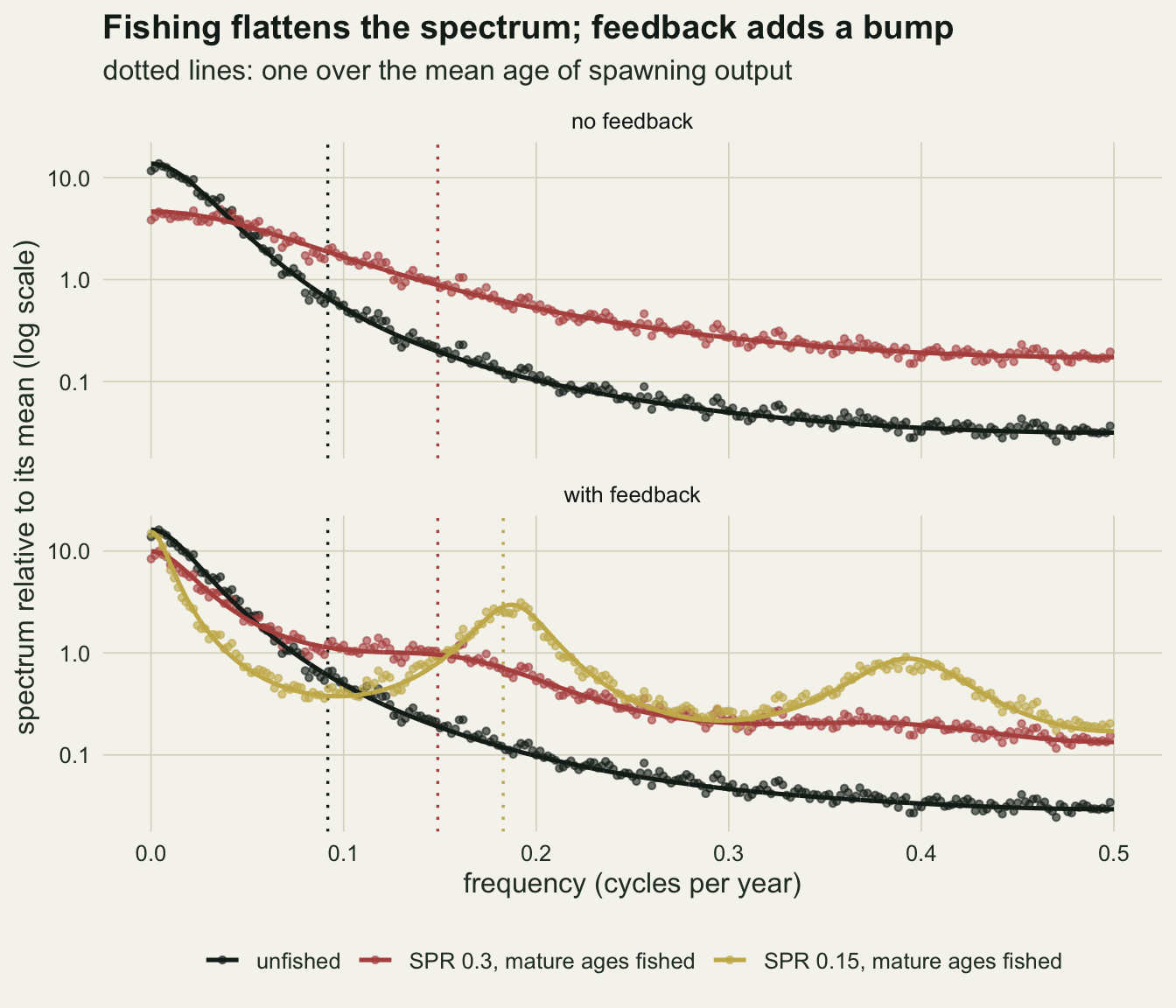

Figure 3: Spectrum of spawning output, relative to its mean level, without and with Beverton-Holt feedback. Lines: closed form; points: smoothed periodogram of 20000 simulated years.

Fifty years of an index

The long runs describe the process. A monitoring programme sees fifty years of a log index with observation error. The detection design fixes the window at 50 years, runs 2000 independent windows for each cell after a burn-in, with feedback on throughout, and uses the standard deviation of the log index within a window as the statistic. Observation error is either absent or normal with standard deviation 0.2 on the log scale, which is modest for a survey index. The unfished reference distribution is simulated twice from independent seeds: one copy supplies the unfished 95th percentile, the other checks that an unfished window exceeds it five per cent of the time.

win_len  <- 50
n_win    <- 2000
win_burn <- 300
obs_grid <- c(0, 0.2)
mc_se_05 <- sqrt(0.05 * 0.95 / n_win)

sim_windows <- function(stk, spr, seed) {
  set.seed(seed)
  eps_w <- matrix(rnorm((win_len + win_burn) * n_win, -sd_rec^2 / 2, sd_rec),
                  nrow = win_len + win_burn)
  f_s   <- f_for_spr(stk, spr, stk$mature)
  f_m   <- matrix(f_s * stk$mature, n_age, n_win)
  run_stock(stk, f_m, rep(1, n_win), rep(TRUE, n_win), eps_w, win_burn)$e_out
}

add_obs <- function(e_mat, obs_sd, seed) {
  set.seed(seed)
  log(e_mat) + matrix(rnorm(length(e_mat), 0, obs_sd), nrow(e_mat))
}

col_sd <- function(y_mat) sqrt(colSums(sweep(y_mat, 2, colMeans(y_mat))^2) / (nrow(y_mat) - 1))

n_eff_est <- function(y_mat, max_lag = 10) {
  y_c <- sweep(y_mat, 2, colMeans(y_mat))
  den <- colSums(y_c^2)
  rho_sq <- vapply(seq_len(max_lag), function(k) {
    (colSums(y_c[1:(win_len - k), ] * y_c[(k + 1):win_len, ]) / den)^2
  }, numeric(ncol(y_mat)))
  win_len / (1 + 2 * rowSums(rho_sq))
}

detect_cell <- function(stk, spr_fish, obs_sd, seeds) {
  e_ref  <- sim_windows(stk, 1, seeds[1])
  e_null <- sim_windows(stk, 1, seeds[2])
  e_fish <- sim_windows(stk, spr_fish, seeds[3])
  y_ref  <- add_obs(e_ref, obs_sd, seeds[4])
  y_null <- add_obs(e_null, obs_sd, seeds[4] + 1)
  y_fish <- add_obs(e_fish, obs_sd, seeds[4] + 2)
  sd_ref <- col_sd(y_ref); sd_null <- col_sd(y_null); sd_fish <- col_sd(y_fish)
  q95    <- quantile(sd_ref, 0.95)
  f_crit <- qf(0.95, win_len - 1, win_len - 1)
  ne_ref <- n_eff_est(y_ref); ne_null <- n_eff_est(y_null); ne_fish <- n_eff_est(y_fish)
  list(sd_ref = sd_ref, sd_fish = sd_fish,
       stats = c(med_ref = median(sd_ref), med_fish = median(sd_fish),
                 exceed = mean(sd_fish > q95), exceed_null = mean(sd_null > q95),
                 naive_size = mean(sd_null^2 / sd_ref^2 > f_crit),
                 naive_power = mean(sd_fish^2 / sd_ref^2 > f_crit),
                 eff_size = mean(sd_null^2 / sd_ref^2 > qf(0.95, ne_null - 1, ne_ref - 1)),
                 eff_power = mean(sd_fish^2 / sd_ref^2 > qf(0.95, ne_fish - 1, ne_ref - 1)),
                 n_eff = median(ne_ref)))
}

det_design <- data.frame(
  label   = c("SPR 0.45, no obs error", "SPR 0.3, no obs error",
              "SPR 0.45, obs sd 0.2", "SPR 0.3, obs sd 0.2"),
  spr     = c(0.45, 0.3, 0.45, 0.3),
  obs     = c(0, 0, 0.2, 0.2))
t_win <- system.time({
  det_out <- lapply(seq_len(nrow(det_design)), function(i) {
    detect_cell(base_stock, det_design$spr[i], det_design$obs[i],
                c(7101, 7202, 7303 + (det_design$spr[i] == 0.3), 7404 + 10 * i))
  })
})[["elapsed"]]
det_tab <- cbind(det_design, t(sapply(det_out, `[[`, "stats")))

sd_long_log <- sd(log(long_run$e_out[, pick(1, "mature", TRUE)]))
var_kept    <- (det_tab$med_ref[2] / sd_long_log)^2
exceed_se   <- sqrt(2) * mc_se_05

Without observation error the median window standard deviation of the unfished log index is 0.117, below the 0.144 of the 20000 year run: squared, the ratio is 0.66, so a typical fifty year window of this slowly wandering series shows about two thirds of its long-run variance. At an SPR of 0.3 the median rises to 0.223, and a fished window lies above the unfished 95th percentile in 0.870 of cases (0.468 at an SPR of 0.45). The independent unfished copy exceeds that percentile in 0.061 of windows against a design value of 0.05; with the percentile itself estimated from 2000 windows the Monte Carlo standard error of that comparison is about 0.007.

Observation error of 0.2 changes the picture. The unfished median becomes 0.234 and the fished median 0.299, because an error of that size is larger than the within-window process variability of the unfished stock. The exceedance probability falls to 0.659 at an SPR of 0.3 and 0.330 at 0.45. These are best cases: they assume the unfished distribution of window standard deviations is known exactly, which in a real comparison it never is.

win_df <- do.call(rbind, lapply(seq_len(nrow(det_design)), function(i) {
  rbind(if (det_design$spr[i] == 0.3)
          data.frame(sd_log = det_out[[i]]$sd_ref, case = "unfished",
                     obs = paste("observation sd", det_design$obs[i])),
        data.frame(sd_log = det_out[[i]]$sd_fish,
                   case = paste("SPR", det_design$spr[i]),
                   obs = paste("observation sd", det_design$obs[i])))
}))
win_df$case <- factor(win_df$case, levels = c("unfished", "SPR 0.45", "SPR 0.3"))

ggplot(win_df, aes(sd_log, colour = case)) +
  geom_density(linewidth = 0.9, adjust = 1.2) +
  facet_wrap(~ obs, ncol = 1) +
  scale_colour_manual(values = c(te_ink, te_gold, te_rust), name = NULL) +
  labs(x = "standard deviation of the log index within a 50-year window",
       y = "density",
       title = "Observation error blurs the change",
       subtitle = "each curve: 2000 windows with Beverton-Holt feedback") +
  theme_datasheet() +
  theme(legend.position = "bottom")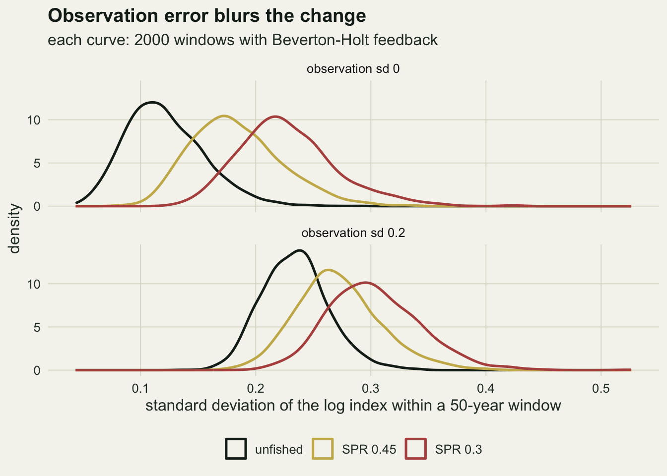

Figure 4: Standard deviation of the log index in 2000 independent 50-year windows, unfished and at two SPRs, without and with observation error.

Testing the change: size before power

The obvious test for two survey series, one fished and one unfished, is the variance ratio F test with 49 and 49 degrees of freedom. It assumes independent years. A spawning output series is anything but independent, so the test’s size has to be measured before its power means anything. The alternative is the same F statistic referred to an F distribution with effective degrees of freedom. For a Gaussian stationary series the variance of the sample variance is inflated by one plus twice the sum of squared autocorrelations, so each series gets an effective length of n over that factor, with the autocorrelations estimated from the series itself up to lag 10. The lag was fixed before running. Size is estimated from pairs of independent unfished series.

sens_design <- data.frame(label = c("maturity at age 8", "steepness 0.5"),
                          age_mat = c(8, 5), h_steep = c(0.7, 0.5))
t_sens <- system.time({
  sens_out <- lapply(seq_len(nrow(sens_design)), function(i) {
    stk_i <- make_stock(sens_design$age_mat[i], sens_design$h_steep[i])
    detect_cell(stk_i, 0.3, 0.2, c(8101, 8202, 8303, 8404) + 1000 * i)$stats
  })
})[["elapsed"]]
sens_tab <- cbind(sens_design, t(sapply(sens_out, identity)))
crash_h5 <- (1 - 0.5) / (4 * 0.5)

test_df <- rbind(
  data.frame(scenario = det_tab$label, test = "naive F", what = "size",
             rate = det_tab$naive_size),
  data.frame(scenario = det_tab$label, test = "naive F", what = "power",
             rate = det_tab$naive_power),
  data.frame(scenario = det_tab$label, test = "effective df", what = "size",
             rate = det_tab$eff_size),
  data.frame(scenario = det_tab$label, test = "effective df", what = "power",
             rate = det_tab$eff_power),
  data.frame(scenario = paste("SPR 0.3, obs sd 0.2,", sens_tab$label), test = "naive F",
             what = "size", rate = sens_tab$naive_size),
  data.frame(scenario = paste("SPR 0.3, obs sd 0.2,", sens_tab$label), test = "naive F",
             what = "power", rate = sens_tab$naive_power),
  data.frame(scenario = paste("SPR 0.3, obs sd 0.2,", sens_tab$label), test = "effective df",
             what = "size", rate = sens_tab$eff_size),
  data.frame(scenario = paste("SPR 0.3, obs sd 0.2,", sens_tab$label), test = "effective df",
             what = "power", rate = sens_tab$eff_power))
mc_se_max <- sqrt(0.25 / n_win)
nc_8 <- vapply(c(1, 0.3), function(s) {
  stk8 <- make_stock(8, 0.7)
  w_8 <- lag_weights(stk8, f_for_spr(stk8, s, stk8$mature) * stk8$mature)
  sum(w_8)^2 / sum(w_8^2)
}, 0)
beta_h5 <- crash_h5 / 0.3
pow_ok  <- c(det_tab$eff_power[det_tab$obs == 0.2], sens_tab$eff_power)
pow_ok_max <- max(pow_ok)

# the effective-df correction on pure white noise of the same length
n_wn <- 20000
set.seed(9105)
wn_a <- matrix(rnorm(win_len * n_wn), win_len)
wn_b <- matrix(rnorm(win_len * n_wn), win_len)
ne_a <- n_eff_est(wn_a)
ne_b <- n_eff_est(wn_b)
wn_neff <- median(ne_a)
wn_size <- mean(col_sd(wn_b)^2 / col_sd(wn_a)^2 > qf(0.95, ne_b - 1, ne_a - 1))

Without observation error the naive test rejects in 0.290 of unfished pairs, against its nominal 0.05. Its power of 0.890 at an SPR of 0.3 is therefore not a power at all. The effective-df version brings the size down to 0.093, still above nominal, with power 0.577. The median estimated effective length of an unfished window is 9.8 years out of 50. The cleaner the index, the more of its variance is slow process variance, and the worse the naive test behaves.

With observation error of 0.2, the error dilutes the autocorrelation and the naive size is 0.092; the effective-df test holds 0.048. Power at an SPR of 0.3 is 0.540 for the naive test and 0.387 for the corrected one, and at 0.45 it is 0.316 and 0.185. The Monte Carlo standard error of any rate here is at most 0.011.

Two sensitivity runs change one design constant each, at an SPR of 0.3 with observation error 0.2. With maturity at age 8 the effective number of cohorts goes from 11.7 unfished to 3.1 at that SPR, and the corrected test reaches power 0.606 at size 0.044 (naive: 0.740 at 0.088). With steepness 0.5 the crash SPR moves to 0.25, so an SPR of 0.3 is close to collapse and the elasticity is 0.83; the corrected test has power 0.466 at size 0.050 (naive: 0.624 at 0.097). Among the cells where the corrected test holds its size (all those with observation error), its highest power is 0.606: a single fifty-year comparison of one fished and one unfished index misses the change in a large share of cases.

test_df$scenario <- factor(test_df$scenario, levels = rev(unique(test_df$scenario)))
test_df$what <- factor(test_df$what, levels = c("size", "power"))

ggplot(test_df, aes(rate, scenario, colour = test, shape = test)) +
  geom_vline(data = data.frame(what = factor("size", levels = c("size", "power")), x0 = 0.05),
             aes(xintercept = x0), linetype = "dashed", colour = te_body, linewidth = 0.6) +
  geom_point(size = 2.8, position = position_dodge(width = 0.5)) +
  facet_wrap(~ what, scales = "free_x") +
  scale_colour_manual(values = c("effective df" = te_forest, "naive F" = te_rust), name = NULL) +
  scale_shape_manual(values = c("effective df" = 16, "naive F" = 17), name = NULL) +
  labs(x = "rejection rate", y = NULL,
       title = "A test that ignores autocorrelation is oversized",
       subtitle = "dashed line: nominal level 0.05") +
  theme_datasheet() +
  theme(legend.position = "bottom", panel.spacing.x = unit(2, "lines"))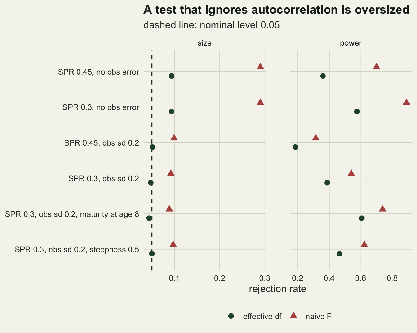

Figure 5: Rejection rates of the variance ratio test between a fished and an unfished 50-year index: size from unfished pairs, power at the stated SPR.

What to report

Report variability as a CV on the arithmetic scale or a standard deviation on the log scale, and say which, together with the effective number of cohorts computed from the weights. For a stock with a maturity schedule, a fecundity curve and a mortality estimate, the no-feedback CV is one line of R and it is the right expectation to set against an observed change: at an SPR of 0.3 in this model it predicts a CV of 0.247 against 0.144 unfished, before any simulation.

State the SPR and the elasticity SPR_crash / SPR next to any variability claim. Down to an SPR of 0.3, where the elasticity is 0.36, the feedback added at most 5.7 per cent to the filter CV; at 0.15 it added 29.8 per cent, and that growth belongs with the early warning literature rather than with age truncation.

When two survey series are compared, report the size of the test alongside its power, estimated for series with the same autocorrelation. The naive variance ratio test was oversized in every cell here, by a factor of up to 5.8 for an index without observation error. An effective degrees of freedom correction held its level once observation error was present and did not without it; the first is two biases roughly cancelling rather than a property of the correction, so the correction should be checked by simulation for the series in hand rather than assumed.

If a spectrum is shown, compare it with the closed-form transfer function for the stock’s own weights before reading a peak as a cycle. In this model the largest spectral value is always at the lowest frequency; a secondary bump near one over the generation time can appear with feedback and a narrow age structure, so read it against the transfer function, not as an independent cycle. Without feedback, the fishing signal is a change in the share of variance at high frequencies.

Honest limits

Recruitment deviations are white. Real recruitment carries environmental autocorrelation, and a red input interacts with the filter: a long-lived stock averages away fast noise but not slow noise, so the contrast between fished and unfished CVs can be expected to shrink as the input reddens; that was not measured. The red noise post covers the unstructured side of that question and nothing here replaces it.

Fishing changes only survival here. Growth, maturity and fecundity at age were held fixed, so there is no fishing-induced evolution, no compensatory growth and no maternal effect of old spawners on larval survival. Selectivity is knife-edge at maturity or flat across ages; a dome-shaped selectivity would sit somewhere between them.

The linearised feedback formula uses relative deviations and ignores the lognormal curvature. With a recruitment log standard deviation of 0.5 that is enough to leave a visible gap near the crash; how the gap depends on the recruitment variance was not measured. The long-run CVs carry block standard errors of the order of 0.003; the ten blocks of a strongly autocorrelated series give a rough standard error, not a precise one.

The detection comparison takes one fished and one unfished series of the same stock, with identical dynamics apart from fishing. A real comparison, like the survey one that motivated this post, sets different species against each other, with different life histories, maturity ages and observation errors, so a difference in variability can arise without fishing at all. The unfished 95th percentile used for exceedance probabilities was known from simulation; in practice it would have to be estimated from few series and the probabilities would be lower. The effective degrees of freedom correction estimated autocorrelations up to lag 10 from fifty points, and the estimate is biased: on pure white noise of the same length the median effective length is 38.0 rather than 50 and the corrected test has size 0.028, so the correction is conservative for white series and liberal for slowly wandering ones (size 0.093 without observation error). With observation error the two biases roughly cancelled. A block bootstrap was not tried.

Steepness, maturity age and observation error were varied one at a time and only at an SPR of 0.3; natural mortality and the recruitment variance were not varied.

References

Hsieh CH, Reiss CS, Hunter JR, Beddington JR, May RM, Sugihara G 2006 Nature 443(7113):859-862 (10.1038/nature05232)

Anderson CNK, Hsieh CH, Sandin SA, Hewitt R, Hollowed A, Beddington J, May RM, Sugihara G 2008 Nature 452(7189):835-839 (10.1038/nature06851)

Bjornstad ON, Nisbet RM, Fromentin JM 2004 Journal of Animal Ecology 73(6):1157-1167 (10.1111/j.0021-8790.2004.00888.x)

Worden L, Botsford LW, Hastings A, Holland MD 2010 Theoretical Population Biology 78(4):239-249 (10.1016/j.tpb.2010.07.004)

Related tutorials

• Stock-recruitment and reference points
• Red noise and extinction risk in a Ricker model
• Spectral analysis of population cycles
• Early warning signals and critical slowing