Early warning signals and critical slowing

Rising lag-1 autocorrelation and variance as a grazed ecosystem approaches a fold bifurcation in R, built from a stochastic model with base stats and a rolling window.

Some ecosystems shift abruptly. A clear lake turns turbid, a grazed grassland collapses to bare ground, a fish stock crashes. When the shift is a fold bifurcation, one stable state collides with an unstable one and disappears, and the system drops to a contrasting state. The unsettling part is that the state variable can look almost unchanged right up to the edge.

Critical slowing down offers a possible warning. As the driver pushes the system towards the fold, the dominant eigenvalue of the linearised dynamics approaches zero, so the system recovers from small perturbations ever more slowly. Slower recovery leaves a fingerprint in the fluctuations: rising lag-1 autocorrelation and rising variance (Scheffer et al. 2009; Carpenter and Brock 2006). This post builds that fingerprint from scratch on a grazing model, using only base stats and a rolling window. It is the setup for a harder question, taken up across this series: when is the rise real, and when is it an artefact of the analysis or of chance.

A grazing model with a fold

We use May’s (1977) grazing model for vegetation biomass x:

\[\frac{dx}{dt} = r\,x\left(1 - \frac{x}{K}\right) - c\,\frac{x^2}{x^2 + h^2}\]

Logistic growth minus a saturating grazing loss. The grazing pressure c is the slow driver. Below a critical value the vegetated state is stable; as c rises the upper equilibrium loses stability at a fold and the system collapses.

r <- 1; K <- 10; h <- 1
f  <- function(x, c) r*x*(1 - x/K) - c*x^2/(x^2 + h^2)

## positive equilibria (f/x = 0) and the fold, by scanning c
g <- function(x, c) r*(1 - x/K) - c*x/(x^2 + h^2)
cgrid <- seq(1.0, 3.2, by = 0.002)
nroot <- sapply(cgrid, function(c){
  xs <- seq(0.001, K, length.out = 6000)
  length(which(diff(sign(g(xs, c))) != 0))
})
c_fold <- cgrid[min(which(nroot <= 1 & cgrid > 2.0))]

Scanning the equilibria puts the fold at c = 2.606. The recovery rate at the upper equilibrium is the slope of the growth function there, and it climbs towards zero as the fold nears:

fp <- function(x, c) r*(1 - 2*x/K) - c*(2*x*h^2)/(x^2 + h^2)^2   # d f / d x
upper_eq <- function(c){ xs <- seq(0.001, K, length.out = 6000)
  idx <- which(diff(sign(g(xs, c))) != 0); max((xs[idx] + xs[idx+1])/2) }
lam <- function(c) fp(upper_eq(c), c)          # dominant eigenvalue (negative)
lam_lo <- lam(1.0); lam_hi <- lam(2.58)
ar1_theory_lo <- exp(lam_lo); ar1_theory_hi <- exp(lam_hi)   # discrete-time AR(1) at unit step

At c = 1 the recovery rate is -0.78 and at c = 2.58 (just short of the fold) it is -0.09. Translated to a lag-1 autocorrelation at unit sampling, that is a rise from 0.46 to 0.91. The theory predicts the direction; the question is whether we can see it in a single noisy realisation.

Simulating an approach to the fold

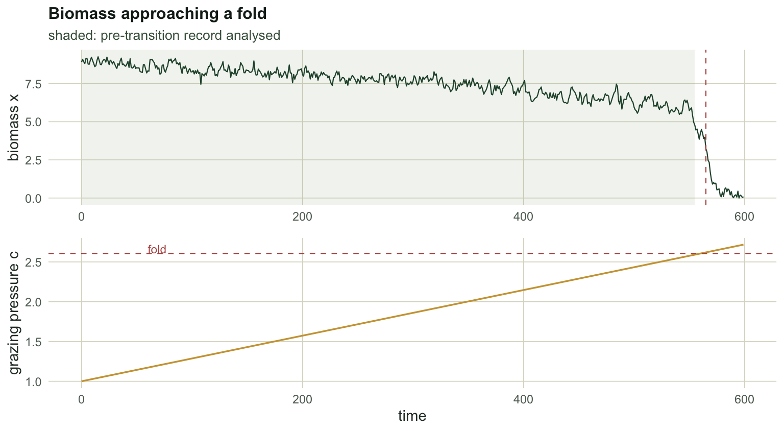
We integrate the model with the Euler-Maruyama scheme, adding a small process noise each step, and ramp c slowly from 1.0 to 2.72 so the system drifts towards the fold and collapses. Sampling is at unit intervals, as an annual monitoring record would be.

sim_grazing <- function(seed, T = 600, dt = 0.01, sigma = 0.30,
                        c0 = 1.0, c1 = 2.72, x0 = 8.9){
  set.seed(seed)
  nstep <- T/dt
  cvec  <- seq(c0, c1, length.out = nstep)
  x <- numeric(nstep); x[1] <- x0
  for(i in 2:nstep){
    xi <- x[i-1]
    x[i] <- xi + f(xi, cvec[i-1])*dt + sigma*sqrt(dt)*rnorm(1)
    if(x[i] < 0.001) x[i] <- 0.001
  }
  keep <- seq(1, nstep, by = 1/dt)
  data.frame(t = (keep-1)*dt, x = x[keep], c = cvec[keep])
}

d <- sim_grazing(seed = 4238)
tr_idx <- which(d$x < 3.5)[1]                 # first crossing into the lower state
t_tr   <- d$t[tr_idx]; c_tr <- d$c[tr_idx]

The system holds near the upper branch, then collapses at t = 565, where the driver has reached c = 2.62: essentially the deterministic fold. Everything up to that point is the pre-transition record we analyse.

Detrending and the rolling window

Early warning indicators are computed on the residuals after removing the slow trend, because the trend itself inflates both variance and autocorrelation. We remove it with a Gaussian kernel smoother (bandwidth a tenth of the record), then slide a window over the residuals and compute the lag-1 autocorrelation and the variance in each window. The AR(1) coefficient here is the order-1 autoregression fit, the standard indicator (Dakos et al. 2012).

seg <- d$x[1:(tr_idx - 10)]; tt <- d$t[1:(tr_idx - 10)]
n <- length(seg)

gauss_detrend <- function(y, bw){
  tg <- seq_along(y)
  trend <- sapply(tg, function(i){ w <- dnorm(tg, i, bw); sum(w*y)/sum(w) })
  y - trend
}
res <- gauss_detrend(seg, 0.10 * n)

win    <- round(0.50 * n)                      # window = half the record
starts <- 1:(n - win + 1)
ar1 <- numeric(length(starts)); vv <- numeric(length(starts))
for(k in seq_along(starts)){
  w <- res[starts[k]:(starts[k] + win - 1)]
  vv[k]  <- var(w)
  ar1[k] <- ar.ols(w, order.max = 1, aic = FALSE,
                   demean = TRUE, intercept = FALSE)$ar[1]
}
tmid <- tt[starts + win %/% 2]

kt_ar  <- cor(seq_along(ar1), ar1, method = "kendall")
kt_var <- cor(seq_along(vv),  vv,  method = "kendall")

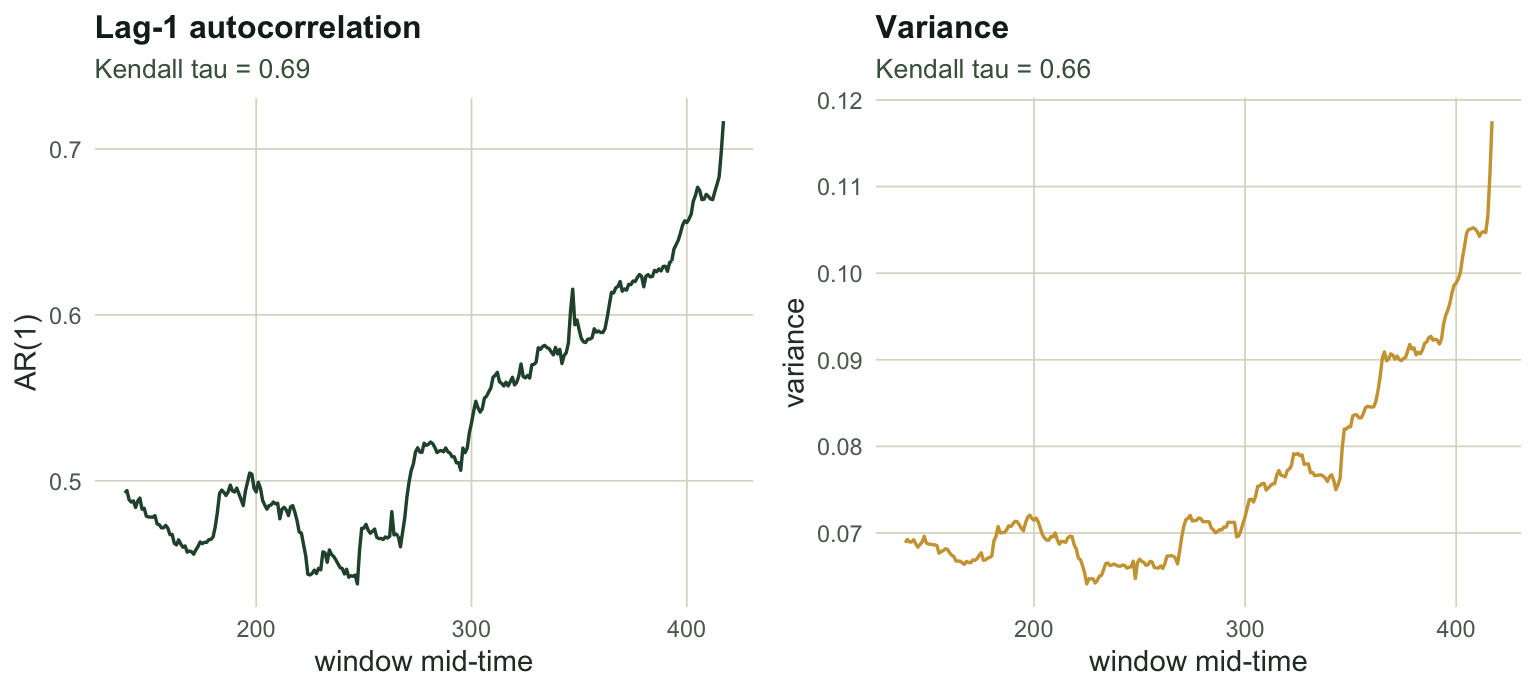
The pre-transition record is 556 points. Both indicators trend up as the fold nears. The lag-1 autocorrelation rises from 0.49 to 0.72 and the variance from 0.069 to 0.118. Summarised as Kendall rank correlations with time, the trend statistics are 0.69 for autocorrelation and 0.66 for variance: strongly positive, the textbook signature of critical slowing.

Figure 1: The grazing model driven slowly towards a fold. Top: biomass holds near the vegetated state, then collapses; the shaded span is the pre-transition record. Bottom: the driver rises to the fold value.

Figure 2: Rolling-window indicators on the detrended residuals. Both the lag-1 autocorrelation and the variance climb as the fold nears; the Kendall rank correlation with time quantifies each trend.

What the rise does and does not tell you

The mechanism is real. As the eigenvalue approaches zero the shocks decay more slowly, so successive observations become more alike (higher autocorrelation) and their spread widens (higher variance). On this idealised record, a long series with a slow, quasi-static approach, the indicators track the theory and the trend statistics are large.

Three cautions temper that. The trend statistics depend on choices, the bandwidth and the window width, that have no objective setting; the next post shows how much those choices move the verdict. The indicators are not specific to a fold; a mere change in the noise, with no bifurcation at all, can push them up too. And the approach here was slow and long, which is what let critical slowing develop; a fast, rate-induced tip can collapse the system with little warning. Most important, a positive Kendall tau is not automatically significant: against a stationary null the tau statistic has a broad distribution, so even this known approach is only marginal. That reckoning is the subject of the checking post in this series. For now, treat a rising indicator as a hypothesis to be tested, not a forecast.

References

• May 1977 Nature 269(5628):471-477 (10.1038/269471a0)
• Carpenter and Brock 2006 Ecology Letters 9(3):311-318 (10.1111/j.1461-0248.2005.00877.x)
• Scheffer et al. 2009 Nature 461(7260):53-59 (10.1038/nature08227)
• Dakos et al. 2012 PLoS ONE 7(7):e41010 (10.1371/journal.pone.0041010)
• Dakos et al. 2015 Philosophical Transactions of the Royal Society B 370(1659):20130263 (10.1098/rstb.2013.0263)

Related tutorials

• Detrending and bandwidth choice in early warning signals
• Spatial early warning signals
• Checking early warning signals
• Detecting ecological thresholds