seg_supF <- function(x, y, grid) {
  fit0 <- lm(y ~ x); rss0 <- sum(fit0$residuals^2); n <- length(y)
  best <- Inf; psi <- NA
  for (p in grid) {
    r <- sum(lm(y ~ x + pmax(x - p, 0))$residuals^2)
    if (r < best) { best <- r; psi <- p }
  }
  list(F = ((rss0 - best) / 1) / (best / (n - 3)), psi = psi)
}
grid <- seq(4, 26, by = 0.2)Testing for an ecological threshold
R
hypothesis testing
ecology tutorial
ggplot2
Deciding whether a threshold is real in base R: the naive break test over-rejects, so bootstrap the null, and do not mistake a smooth curve for a kink.
Corrected 27 September 2026: the closing section said the data support the choice between a threshold and a smooth bend only weakly; in the worked example AIC separates them clearly once the smooth curve is fitted, and the section now says so.
The previous post fitted a breakpoint by profiling the residual sum of squares. That procedure always returns a minimum, so a good broken-stick fit is not by itself evidence that a threshold exists. This post asks the harder question: is the break real, or would a straight line have done?
The tempting shortcut is to fit the two-piece model, read the p-value of the slope-change term, and call anything below 0.05 a threshold. That test is not valid. Under the hypothesis of no break the breakpoint is not a parameter of the model at all, so it is estimated from the noise, and the usual F reference does not hold. The fix is to build the null distribution by simulation, and to remember that rejecting a straight line is not the same as finding a kink.
Why the naive p-value is wrong
The statistic itself is fine: at each candidate breakpoint, compare the two-piece fit with the straight line by an F ratio, and take the largest F over all candidates. This maximised value is the natural test statistic.
The trouble is the reference. An ordinary F statistic for one added term follows an F distribution with one and \(n - 3\) degrees of freedom. But this F was maximised over every candidate breakpoint, so it is systematically larger than a single F even when nothing is going on. Simulate straight-line data with no break, run the procedure, and read the naive p-value each time.
set.seed(4199)
Rrep <- 2000; n <- 80
naive_p <- numeric(Rrep)
for (r in seq_len(Rrep)) {
  x <- runif(n, 0, 30)
  y <- 20 - 0.15 * x + rnorm(n, 0, 3)         # a plain line, no break
  naive_p[r] <- pf(seg_supF(x, y, grid)$F, 1, n - 3, lower.tail = FALSE)
}
rej_naive <- mean(naive_p < 0.05)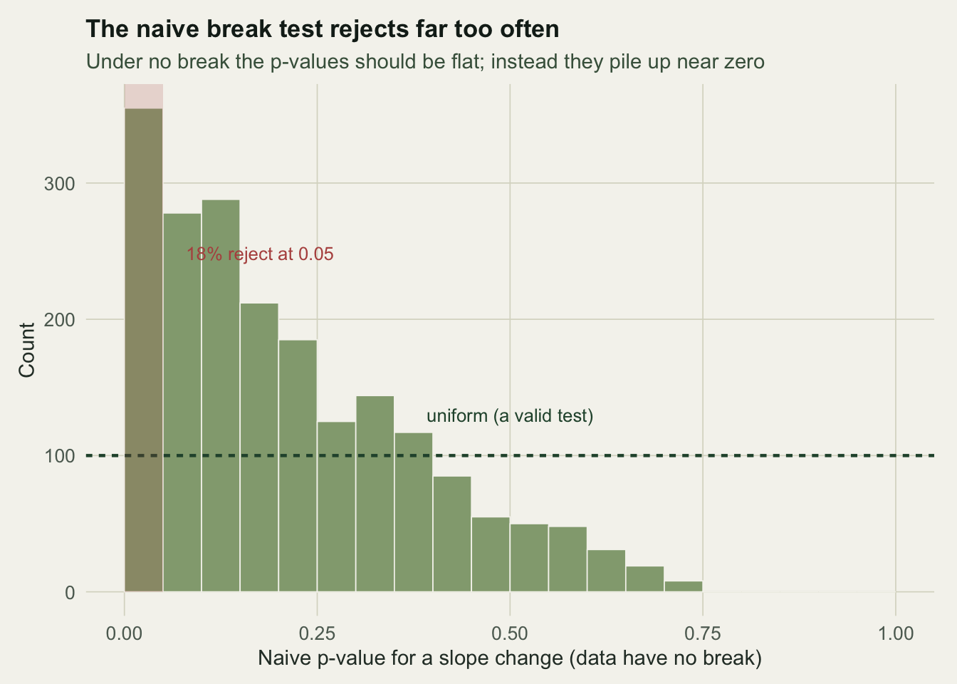
The p-values in Figure 1 are not flat. They crowd towards zero, and about 18% fall below 0.05 rather than the 5% a valid test would give. Read literally, that is how often the naive break test would announce a threshold in data sets that have none.
A null distribution by bootstrap
The repair is to compare the observed statistic against its own null distribution rather than an off-the-shelf F. Fit the straight line, treat that as the truth, simulate new responses from it, and recompute the maximised F each time. Here is a data set with a genuine break to test.
set.seed(781)
n <- 100
x <- runif(n, 0, 30); psi0 <- 14
y <- 18 + 0.10 * x - 0.80 * pmax(x - psi0, 0) + rnorm(n, 0, 2.5)
obs <- seg_supF(x, y, grid)
naive_p_obs <- pf(obs$F, 1, n - 3, lower.tail = FALSE)

fit0 <- lm(y ~ x); sig0 <- summary(fit0)$sigma
set.seed(55)
B <- 1200
null_F <- replicate(B, seg_supF(x, fitted(fit0) + rnorm(n, 0, sig0), grid)$F)
p_boot <- (1 + sum(null_F >= obs$F)) / (B + 1)
crit_boot  <- quantile(null_F, 0.95)
crit_naive <- qf(0.95, 1, n - 3)
size_naive <- mean(null_F > crit_naive)     # the naive test's true size
The maximised F here is 57.4, which the F table would call significant at about \(2.1 \times 10^{-11}\). The bootstrap agrees that the break is real but is far more measured: its p-value is 0.001. The difference is entirely in the threshold. A valid 5% test needs an F above 6.6 (the 95th percentile of the null distribution), whereas the naive table uses 3.9. Using that lower bar, the actual rejection rate under no break is 17%, matching the 18% from the direct simulation above. Two routes, one conclusion: the F table is roughly three to four times too generous.
A significant test is not a threshold
There is a deeper limit, and it is the honest note of the cluster. The break test asks whether a straight line is adequate. It does not ask whether the true shape is a kink. A smooth curve that bends also fails the straight-line test, and it will fail it emphatically.
set.seed(4299)
n <- 90
x <- runif(n, 0, 30)
y <- 30 * x / (6 + x) + rnorm(n, 0, 2.2)        # smooth saturation, no kink
sm <- seg_supF(x, y, grid)
naive_p_smooth <- pf(sm$F, 1, n - 3, lower.tail = FALSE)

fit_seg <- lm(y ~ x + pmax(x - sm$psi, 0))
fit_mm  <- nls(y ~ SSmicmen(x, Vm, K))          # the smooth alternative
aic_seg <- AIC(fit_seg) + 2                      # +2 for the estimated breakpoint
aic_mm  <- AIC(fit_mm)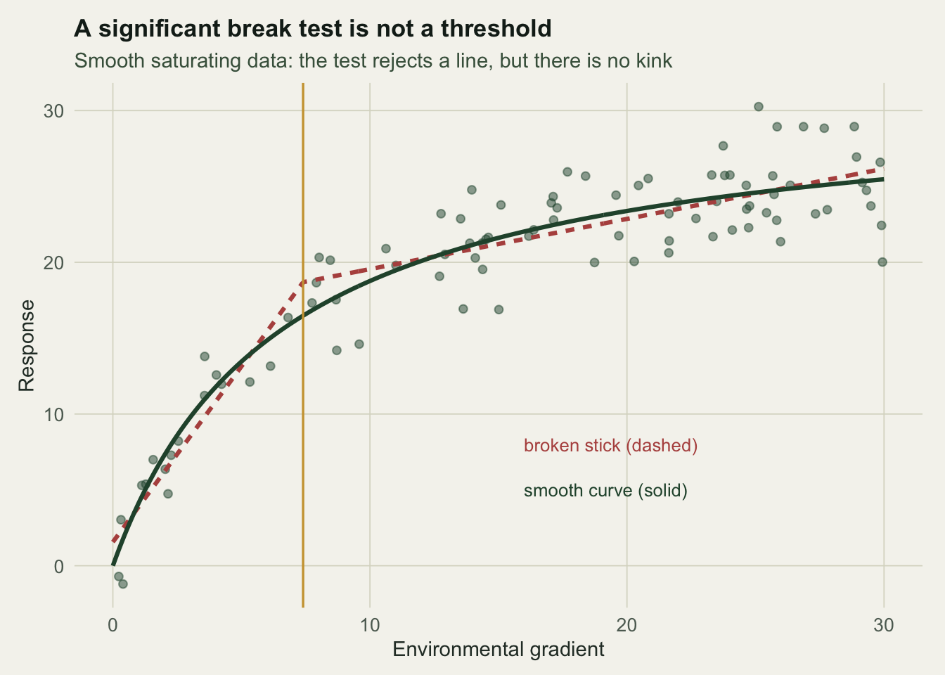
The data in Figure 2 are a smooth saturating curve with no breakpoint anywhere. The maximised F is 122, and the naive p-value is about \(3 \times 10^{-18}\): an overwhelming vote against the straight line. A practitioner who compares only a line with a broken stick will report a sharp threshold. But when the smooth saturating curve is fitted as well, AIC prefers it by about 12.4 points, revealing the apparent break as a gentle bend.
The honest limit
A break test controls a single decision: is a straight line enough? Do not run it with the F table, which is calibrated for a fixed breakpoint and rejects three to four times too often once the breakpoint is estimated; build the null distribution by simulation instead. And once a line is rejected, the work is not finished. Ask AIC, or a smooth alternative, whether the response truly turns at a point or simply curves. Distinguishing a genuine threshold from a smooth bend is a choice between shapes, and the break test alone cannot make it: it takes a smooth alternative fitted alongside, as here, where AIC separated the two by about 12 points. The next post carries the threshold idea into count and presence data, where the same distinction between a step and a slope has to be made explicitly.
References
- Toms JD, Lesperance ML 2003. Ecology 84(8):2034-2041 (10.1890/02-0472)
- Toms JD, Villard MA 2015. Avian Conservation and Ecology 10(1):2 (10.5751/ACE-00715-100102)
- Davies RB 1987. Biometrika 74(1):33-43 (10.1093/biomet/74.1.33)
- Andrews DWK 1993. Econometrica 61(4):821-856 (10.2307/2951764)
- Muggeo VMR 2003. Statistics in Medicine 22(19):3055-3071 (10.1002/sim.1545)