Threshold regression with a GLM

Threshold models for count data in base R: profile a Poisson GLM for the breakpoint, tell a slope change from an abrupt regime shift, and resist extra breakpoints.

The first two posts fitted and tested a breakpoint for a Gaussian response. Ecological data are more often counts or presences, and the same shape appears there: an abundance that holds steady then falls once a stressor passes a threshold, a species that occupies sites up to a limit of temperature or forest cover and then drops out. The hinge idea carries over directly, because a generalised linear model has a linear predictor, and a breakpoint is just a term in it. Two further questions become sharper once the response is a count: whether the threshold is a change of slope or an abrupt jump, and how many breakpoints to allow.

A threshold inside a Poisson GLM

Here is a count that is flat below a temperature threshold and declines above it, on the log scale where the Poisson model works.

set.seed(4200)
n <- 200
temp <- runif(n, 0, 30); psi_true <- 15
count <- rpois(n, exp(2.5 + 0.0 * temp - 0.12 * pmax(temp - psi_true, 0)))

The reflex model puts one slope on the log mean.

fit_naive <- glm(count ~ temp, family = poisson)
naive_slope <- coef(fit_naive)[["temp"]]

That single log slope is -0.05, a gentle decline that describes the whole range as if abundance fell steadily from the start. To fit the threshold, profile the breakpoint on the deviance, exactly as before but with glm in place of lm.

dev_at <- function(p) deviance(glm(count ~ temp + pmax(temp - p, 0), family = poisson))
grid <- seq(5, 25, by = 0.25)
psi_hat <- grid[which.min(vapply(grid, dev_at, numeric(1)))]
hinge <- pmax(temp - psi_hat, 0)
fit_thr <- glm(count ~ temp + hinge, family = poisson)
cf <- coef(fit_thr)
below_log <- cf[["temp"]]
above_log <- cf[["temp"]] + cf[["hinge"]]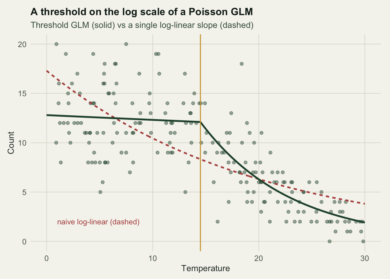

Figure 1: A Poisson count with a threshold in temperature. The threshold GLM (solid) is flat then falls at the breakpoint; a single log-linear slope (dashed) smears the decline across the whole gradient.

The profiled breakpoint sits at 14.5, close to the true 15. Below it the log mean is essentially flat (-0.004); above it the log mean falls by -0.12 per degree, which multiplies the expected count by about 0.55 over each five degrees past the threshold. The threshold model lowers the AIC by roughly 77 once the breakpoint is counted (Figure 1). The interpretation is now ecological rather than an averaged slope: the community is unaffected up to 14.5 degrees, then loses individuals steeply.

A slope change or a regime shift?

A breakpoint can mean two different things. In a continuous threshold the response is unbroken at the join and only its slope changes, a hinge. In a discontinuous threshold the response jumps to a new level, a step. These are different ecological claims: a gradual turning point where a decline begins, against a regime shift where the system moves to a new state. They need different terms, and the data can usually tell them apart.

The data below are a genuine level shift, a count that drops abruptly to a lower state above the threshold.

set.seed(4210)
x <- runif(200, 0, 30); psi0 <- 15
yb <- rpois(200, exp(2.4 - 1.1 * (x > psi0)))
g <- seq(5, 25, by = 0.25)
dev_cont <- function(p) deviance(glm(yb ~ x + pmax(x - p, 0), family = poisson))       # slope change
dev_step <- function(p) deviance(glm(yb ~ x + as.numeric(x > p), family = poisson))    # level shift
pc <- g[which.min(vapply(g, dev_cont, numeric(1)))]
ps <- g[which.min(vapply(g, dev_step, numeric(1)))]
fit_cont <- glm(yb ~ x + pmax(x - pc, 0), family = poisson)
fit_step <- glm(yb ~ x + as.numeric(x > ps), family = poisson)
aic_cont <- AIC(fit_cont) + 2
aic_step <- AIC(fit_step) + 2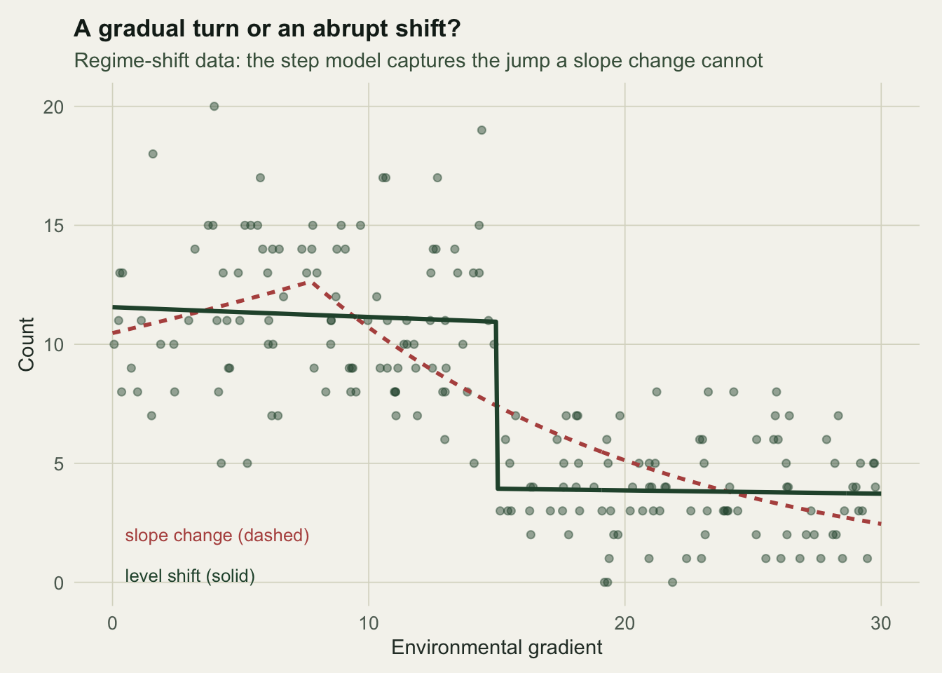

Figure 2: Regime-shift data. The step model (solid) places the jump correctly; the slope-change model (dashed) cannot represent a jump and settles on a misleading breakpoint elsewhere.

The step model puts its jump at 15, right on the true shift, and estimates a drop of -1.02 on the log scale, a fall to about 0.36 of the earlier level. The slope-change model cannot bend sharply enough, so it lands on a breakpoint at 7.8 and fits worse: its AIC is higher by about 58.2 (Figure 2). Forcing the wrong type does more than fit poorly; it tells the wrong story and reports a breakpoint in the wrong place. The choice between a hinge and a step is a modelling decision, guided by AIC and by whether the ecology is a turning point or a state change.

How many breakpoints?

One breakpoint may not be the end of it, and this is where threshold models overfit. Adding breakpoints can only lower the deviance, just as adding hidden states or predictors always improves the in-sample fit, so the count of breakpoints has to be chosen rather than maximised. On the single-threshold data from the first section, fit zero, one, and two breakpoints and let AIC and BIC weigh the extra parameters.

dev0 <- deviance(glm(count ~ temp, family = poisson))
dev1 <- deviance(fit_thr)
g2 <- seq(6, 24, by = 1)
best2 <- Inf
for (a in g2) for (b in g2) if (b > a + 1) {
  d <- deviance(glm(count ~ temp + pmax(temp - a, 0) + pmax(temp - b, 0), family = poisson))
  if (d < best2) best2 <- d
}
dev2 <- best2
aic_k <- c(dev0 + 2 * 2, dev1 + 2 * 4, dev2 + 2 * 6)   # k = 2, 4, 6 parameters
bic_k <- c(dev0 + log(n) * 2, dev1 + log(n) * 4, dev2 + log(n) * 6)

The deviances fall from 263.3 to 182 to 180: adding a second breakpoint helps a little, as it always will. But the second breakpoint buys almost nothing real, so AIC rises again at two (267, 190, 192), and BIC, which penalises more heavily, rejects it firmly (274, 203, 212). Both select the one true breakpoint. With enough joins a broken line can trace any wiggle, so treat the number of breakpoints as a quantity to select, and prefer the simplest model the data support.

The honest limit

A GLM makes threshold models available for the responses ecology actually records, but it does not settle the shape. Whether the response changes slope or jumps, and how many times, are choices the analyst imposes; the data reward the better choice through AIC but rarely force it. The closing post checks a fitted threshold model directly: how honest its breakpoint interval is, how sensitive the story is to the assumed shape, and why a good fit is never proof that the threshold is where, or what, the model says.

References

• Ficetola GF, Denoel M 2009. Ecography 32(6):1075-1084 (10.1111/j.1600-0587.2009.05571.x)
• Toms JD, Lesperance ML 2003. Ecology 84(8):2034-2041 (10.1890/02-0472)
• Muggeo VMR 2003. Statistics in Medicine 22(19):3055-3071 (10.1002/sim.1545)
• Bai J, Perron P 1998. Econometrica 66(1):47-78 (10.2307/2998540)
• Bolker BM 2008. Ecological Models and Data in R. Princeton University Press (ISBN 978-0-691-12522-0)

Related tutorials

• Segmented regression for a breakpoint
• Testing for an ecological threshold
• Checking a threshold model
• GLMs for count and abundance data