set.seed(4231)
n <- 90
x <- runif(n, 0, 30); psi0 <- 14
y <- 18 + 0.10 * x - 0.55 * pmax(x - psi0, 0) + rnorm(n, 0, 2.5)
grid <- seq(4, 26, by = 0.2)
psi_hat <- grid[which.min(vapply(grid, function(p) sum(lm(y ~ x + pmax(x - p, 0))$residuals^2), numeric(1)))]
fit_line <- lm(y ~ x)
fit_thr  <- lm(y ~ x + pmax(x - psi_hat, 0))

line_curv <- summary(lm(residuals(fit_line) ~ poly(fitted(fit_line), 2)))$coefficients[3, 4]
thr_curv <- summary(lm(residuals(fit_thr) ~ poly(fitted(fit_thr), 2)))$coefficients[3, 4]Checking a threshold model
R
model diagnostics
ecology tutorial
ggplot2
Checking a fitted threshold in base R: read the residuals, see why the Wald breakpoint interval undercovers, and test the threshold under a different shape.
A fitted threshold model is persuasive. It reports a breakpoint to two decimals, draws two clean lines, and lowers the AIC against a straight line. This closing post is about the checks that stand between that output and a claim. There are three: whether the two-piece shape actually fits, whether the interval around the breakpoint is honest, and how much the whole story depends on assumptions the data cannot settle. Each mirrors the diagnostic that closed the earlier method clusters, and the last is the familiar limit of this one.
Do the residuals still carry a pattern?
The first check is the cheapest. If a straight line is wrong and a broken stick is right, the line will leave structure in its residuals and the broken stick will not. Fit both and look.
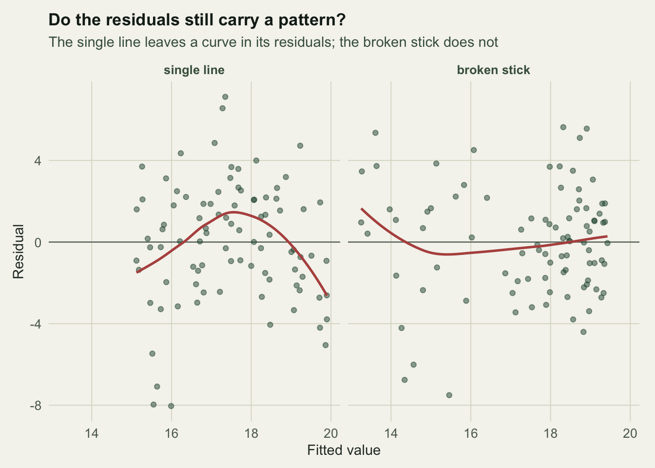
A quadratic fitted to the line’s residuals has a highly significant curvature term (p \(3.5 \times 10^{-4}\)), the fingerprint of a bend the line cannot follow. The same term on the broken stick’s residuals is not significant (p 0.17): the two-piece shape has absorbed the structure (Figure 1). If the broken stick’s residuals still curved, that would be a warning that the true shape is smooth rather than kinked, the distinction from the previous post.
Is the breakpoint interval honest?
The breakpoint comes with a standard error, and the quick one is not trustworthy. The usual Wald interval treats the breakpoint like any coefficient, but its sampling distribution is skewed and its quick standard error is too small, so the interval is too narrow. A profile interval, the set of breakpoints whose fit is statistically indistinguishable from the best, is wider and closer to honest.
fit_bs <- function(x, y, grid) {
  n <- length(y)
  rss <- vapply(grid, function(p) sum(lm(y ~ x + pmax(x - p, 0))$residuals^2), numeric(1))
  psi <- grid[which.min(rss)]; rss_min <- min(rss); sig2 <- rss_min / (n - 3)
  aug <- lm(y ~ x + pmax(x - psi, 0) + as.numeric(x > psi))    # Muggeo's augmented fit
  se_psi <- summary(aug)$coefficients[4, 2] / abs(coef(aug)[[3]])
  wald <- psi + c(-1, 1) * 1.96 * se_psi
  prof <- range(grid[rss <= rss_min + sig2 * qchisq(0.95, 1)])
  list(wald = wald, prof = prof)
}set.seed(4201)
Rrep <- 1500; n <- 80; psi0 <- 14
cov_wald <- 0; cov_prof <- 0
for (r in seq_len(Rrep)) {
x <- runif(n, 0, 30)
y <- 18 + 0.10 * x - 0.60 * pmax(x - psi0, 0) + rnorm(n, 0, 3)
f <- fit_bs(x, y, grid)
cov_wald <- cov_wald + (psi0 >= f$wald[1] && psi0 <= f$wald[2])
cov_prof <- cov_prof + (psi0 >= f$prof[1] && psi0 <= f$prof[2])
}
cov_wald <- cov_wald / Rrep; cov_prof <- cov_prof / Rrep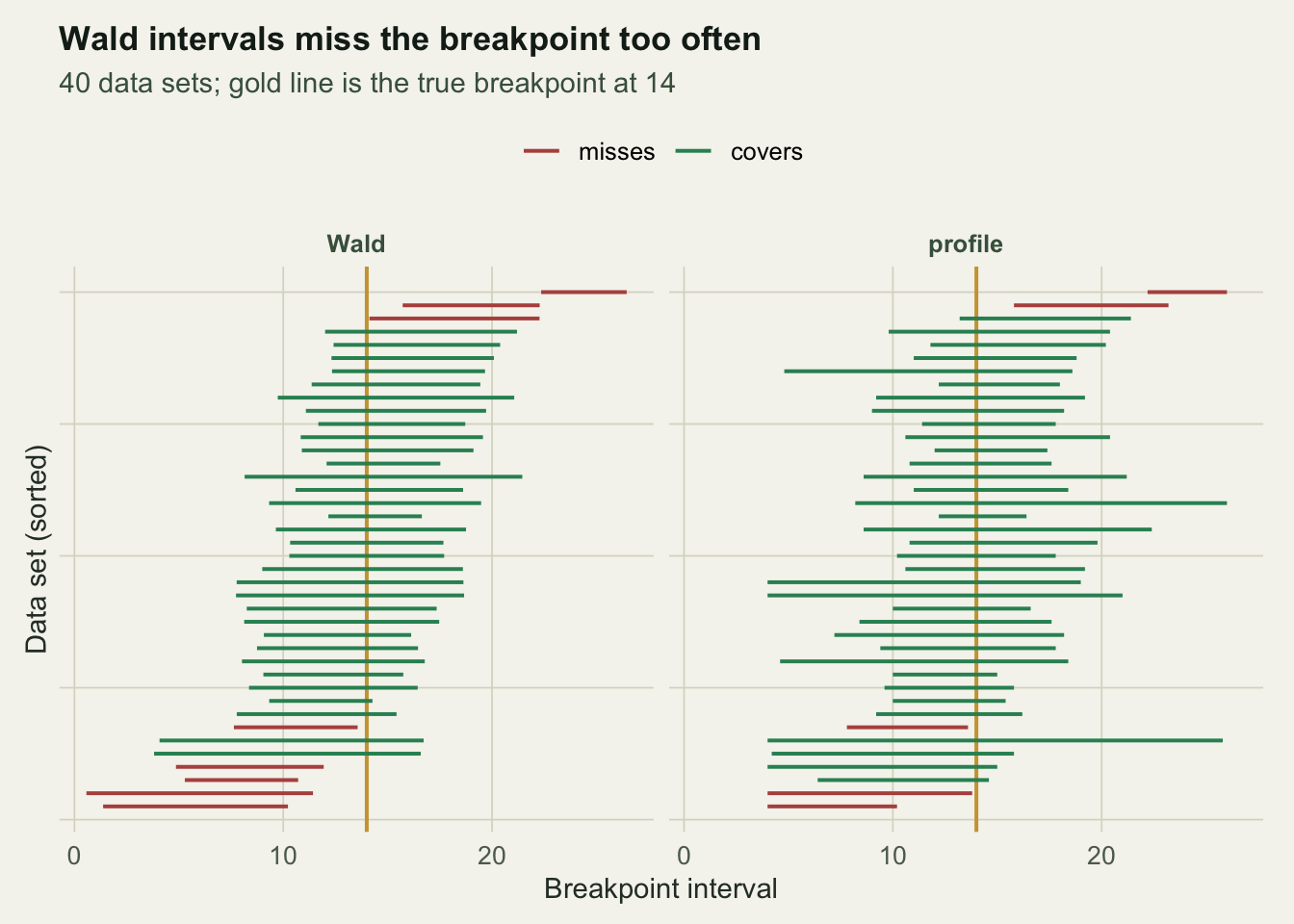
Across 1500 data sets the Wald interval covers the true breakpoint only 79% of the time, well short of the nominal 95%, while the profile interval reaches 93% (Figure 2). The Wald interval is not merely imperfect; it is confidently wrong about a value it barely constrains. Report the profile interval, or a bootstrap interval as in the first post, and never the quick standard error alone.
How much does the threshold depend on assumptions?
The last check is the honest limit of the cluster. A breakpoint is reported as a number, but that number is conditional on choices the data support only weakly: the assumed shape, the number of breakpoints, and the noise. Change any of them and the threshold moves.
set.seed(9014)
n <- 120
x <- runif(n, 0, 30); psi0 <- 14
y <- 18 + 0.10 * x - 0.70 * pmax(x - psi0, 0) + rnorm(n, 0, 2.5)
psi_cont <- grid[which.min(vapply(grid, function(p) sum(lm(y ~ x + pmax(x - p, 0))$residuals^2), numeric(1)))]
psi_step <- grid[which.min(vapply(grid, function(p) sum(lm(y ~ x + as.numeric(x > p))$residuals^2), numeric(1)))]

est_psi <- function(xx, yy) {
  g <- seq(4, 26, by = 0.25)
  g[which.min(vapply(g, function(p) sum(lm(yy ~ xx + pmax(xx - p, 0))$residuals^2), numeric(1)))]
}
set.seed(31)
boot_psi <- replicate(1500, { i <- sample.int(n, n, replace = TRUE); est_psi(x[i], y[i]) })
bci <- quantile(boot_psi, c(0.025, 0.975))
On one data set, a continuous slope-change model puts the threshold at 15.4, near the true 14. Assume instead that the response steps to a new level, and the same data place the threshold at 20, more than four units away. The noise adds its own width: the bootstrap interval for the continuous estimate runs from 12.5 to 17.8. So a single reported breakpoint stands for a range that depends on the assumed shape and on chance, and the number of breakpoints (from the previous post) is a further choice on top.
The honest limit
A threshold model does not read a breakpoint out of nature. It fits the breakpoint of a shape you chose, with an interval that only the slower methods report honestly, and a location that shifts when the shape or the count changes. The disciplined summary is a checked model: residuals without remaining structure, a profile or bootstrap interval rather than the quick one, and a sensitivity range across the shapes and counts the data cannot rule out. That last step is the same move made throughout these clusters, where an unverifiable assumption is turned into a stated magnitude rather than hidden inside a point estimate: the E-value for an unmeasured confounder, the delta shift for missing-data mechanisms, the reference frame for compositional change, the extrapolation for a nonlinear form. A threshold is not a fact the data hand over; it is a claim, conditional on a shape, and worth only as much as the checks behind it.
References
- Muggeo VMR 2017. Australian and New Zealand Journal of Statistics 59(3):311-322 (10.1111/anzs.12200)
- Muggeo VMR 2003. Statistics in Medicine 22(19):3055-3071 (10.1002/sim.1545)
- Toms JD, Lesperance ML 2003. Ecology 84(8):2034-2041 (10.1890/02-0472)
- Ficetola GF, Denoel M 2009. Ecography 32(6):1075-1084 (10.1111/j.1600-0587.2009.05571.x)
- Bolker BM 2008. Ecological Models and Data in R. Princeton University Press (ISBN 978-0-691-12522-0)