set.seed(4198)
n <- 120
nitrogen <- runif(n, 0, 30)             # kg N/ha/yr
psi_true <- 12                          # the real breakpoint
richness <- 25 + 0.10 * nitrogen - 0.90 * pmax(nitrogen - psi_true, 0) +
  rnorm(n, 0, 2.5)
dat <- data.frame(nitrogen, richness)Segmented regression for a breakpoint
R
regression
ecology tutorial
ggplot2
Fit a broken-stick model to an ecological threshold in base R: profile the residual sum of squares to place the breakpoint, and see why one line misleads.
Many ecological responses do not bend gently. A grassland loses forbs once nitrogen deposition passes a level the soil can buffer; a stream community collapses above a sediment load; edge effects fade at a fixed distance into a forest. In each case the relationship is roughly linear on either side of a breakpoint, and the breakpoint itself is the quantity of interest. A single straight line cannot represent that shape, and fitting one does not just lose detail: it produces a slope that describes neither side.
This post fits a two-piece (“broken-stick”) model in base R, locates the breakpoint by profiling the residual sum of squares, and reads off the slope on each side. The honest limit at the end is the theme of the whole cluster: a breakpoint is a feature of the model you chose, and its location carries real uncertainty.
A threshold response
Here is a simulated richness response to nitrogen deposition. Below a threshold the community is stable; above it, richness falls.
The generating slope is a near-flat 0.10 below the threshold and a declining -0.80 above it, with the join at 12.
Why one line misleads
The reflex is a single linear model.
fit_lin <- lm(richness ~ nitrogen, data = dat)
lin_slope <- coef(fit_lin)[["nitrogen"]]
lin_r2 <- summary(fit_lin)$r.squared
That line has a slope of -0.51 and an R-squared of 0.59. The number looks like a tidy answer, but it is an average of two regimes that do not exist together anywhere in the data. Below the threshold the response is flat; above it, it drops much more steeply than the single slope suggests. Reporting -0.51 as “the effect of nitrogen” describes a mixture, not a mechanism.
Fitting a broken stick
A continuous two-piece model adds one hinge term. For a candidate breakpoint \(\psi\), the term \((x - \psi)_+\) equals \(x - \psi\) above \(\psi\) and zero below it, so the model
\[y = \beta_0 + \beta_1 x + \beta_2 (x - \psi)_+ + \varepsilon\]
is ordinary least squares given \(\psi\): the slope is \(\beta_1\) below the breakpoint and \(\beta_1 + \beta_2\) above it. The one awkward parameter is \(\psi\), which enters non-linearly. The direct approach is to profile it: fit the linear model at every candidate breakpoint and keep the value that minimises the residual sum of squares.
rss_at <- function(p) {
  hinge <- pmax(dat$nitrogen - p, 0)
  sum(lm(richness ~ nitrogen + hinge, data = dat)$residuals^2)
}
grid <- seq(3, 27, by = 0.1)
rss_grid <- vapply(grid, rss_at, numeric(1))
psi_hat <- optimize(rss_at, lower = grid[which.min(rss_grid)] - 0.2,
                    upper = grid[which.min(rss_grid)] + 0.2)$minimum

hinge <- pmax(dat$nitrogen - psi_hat, 0)
fit_seg <- lm(richness ~ nitrogen + hinge, data = dat)
cf <- coef(fit_seg)
below_slope <- cf[["nitrogen"]]
above_slope <- cf[["nitrogen"]] + cf[["hinge"]]
seg_r2 <- summary(fit_seg)$r.squared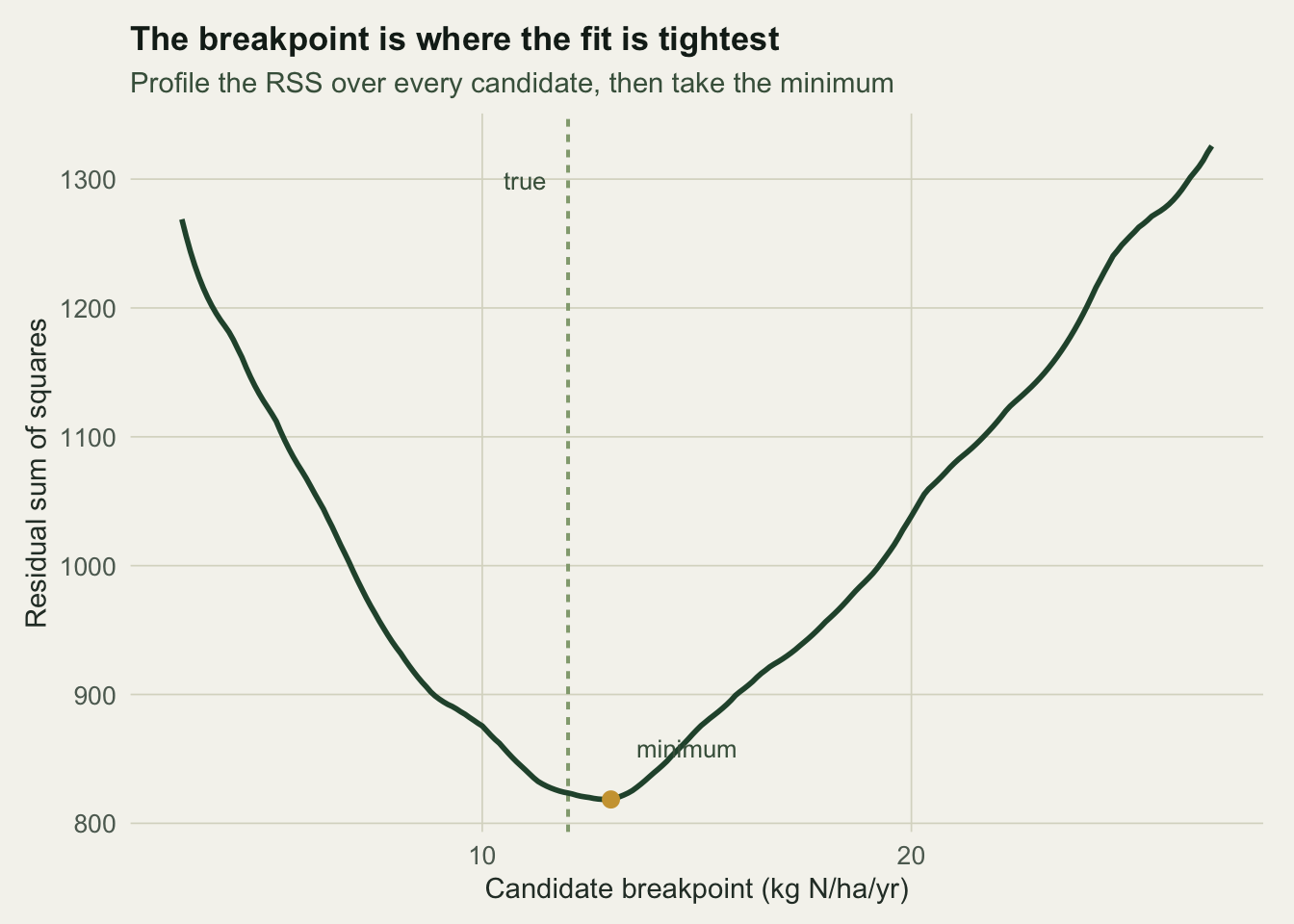
The profile in Figure 1 has a single clear valley. Its minimum puts the breakpoint at 13 kg N/ha/yr, close to the true 12. The fitted slopes are 0.17 below the breakpoint and -0.93 above it, recovering the flat-then-declining shape. The two-piece model explains far more of the scatter than the line (R-squared 0.77 against 0.59), and once the extra breakpoint parameter is counted its AIC is lower by about 66.
How uncertain is the breakpoint?
The breakpoint is an estimate, not a landmark, and its standard error is not one of the numbers lm prints. A case bootstrap gives an honest interval: resample rows, refit the whole procedure, and collect the breakpoint each time.
est_psi <- function(x, y) {
  f <- function(p) sum(lm(y ~ x + pmax(x - p, 0))$residuals^2)
  g <- seq(3, 27, by = 0.25)
  p0 <- g[which.min(vapply(g, f, numeric(1)))]
  optimize(f, lower = p0 - 0.5, upper = p0 + 0.5)$minimum
}
set.seed(101)
boot_psi <- replicate(2000, {
  i <- sample.int(n, n, replace = TRUE)
  est_psi(dat$nitrogen[i], dat$richness[i])
})
psi_ci <- quantile(boot_psi, c(0.025, 0.975))
psi_se <- sd(boot_psi)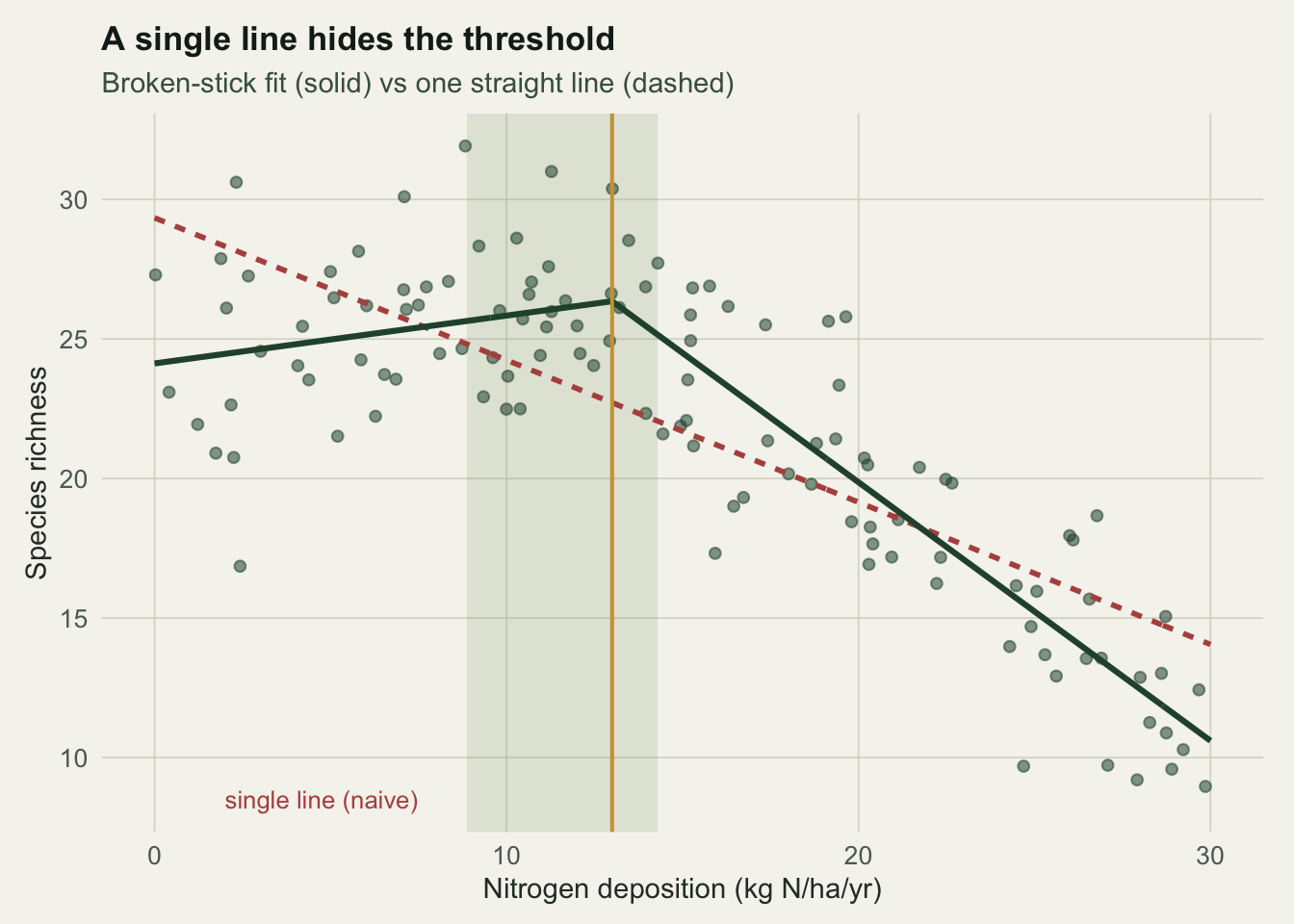
The bootstrap puts the breakpoint at roughly 8.9 to 14.3 kg N/ha/yr (standard error about 1.2), shown as the band in Figure 2. The interval covers the true value but spans several units: a study reporting a threshold of “13” without that band overstates how precisely the join is known.
The honest limit
Two cautions carry into the rest of this cluster. First, the breakpoint is a property of a model that assumes a break; the profile will always return a minimum, even for data with no genuine threshold, so a low RSS at some \(\psi\) is not evidence that a threshold exists. Testing whether a break is real is a separate problem, because under the no-break hypothesis the breakpoint is not identified and the usual test on \(\beta_2\) is invalid; that is the subject of the next post. Second, a sharp join is one shape among several. A smooth curve can fit a threshold-looking scatter just as well, and telling a genuine break from a gradual bend is a question the data alone rarely settle.
References
- Toms JD, Lesperance ML 2003. Ecology 84(8):2034-2041 (10.1890/02-0472)
- Muggeo VMR 2003. Statistics in Medicine 22(19):3055-3071 (10.1002/sim.1545)
- Muggeo VMR 2008. R News 8(1):20-25 (ISSN 1609-3631)
- Hudson DJ 1966. Journal of the American Statistical Association 61(316):1097-1129 (10.1080/01621459.1966.10482198)
- Bolker BM 2008. Ecological Models and Data in R. Princeton University Press (ISBN 978-0-691-12522-0)