Checking early warning signals

Surrogate tests, false-positive rates and the necessary-not-sufficient limit of early warning signals in R, showing why a rising indicator is a hypothesis, not a forecast.

The earlier tutorials in this series showed indicators that rise before a fold: lag-1 autocorrelation and variance in time, the same on residuals under different analyst choices, and variance and Moran’s I in space. Each ended on the same warning: a rising indicator is a hypothesis, not a forecast. This post does the reckoning. It asks three questions of any early warning claim. Is the rise distinguishable from chance? How often does the test cry wolf when nothing is happening? And can the indicator rise without a transition, or a transition happen without the indicator. The answers are sobering, and they are the reason to treat these tools as a screen rather than a prediction.

The shared machinery

We reuse the collapsing grazing series and the same rolling-window indicators. The lag-1 autocorrelation is computed with the direct order-1 estimator, which matches ar.ols exactly and is quicker inside a Monte Carlo loop.

r <- 1; K <- 10; h <- 1
f <- function(x, c) r*x*(1 - x/K) - c*x^2/(x^2 + h^2)

gauss_detrend <- function(y, bw){ tg <- seq_along(y)
  trend <- sapply(tg, function(i){ w <- dnorm(tg, i, bw); sum(w*y)/sum(w) }); y - trend }
ar1_fast <- function(w){ w <- w - mean(w); L <- length(w)
  sum(w[2:L]*w[1:(L-1)]) / sum(w[1:(L-1)]^2) }              # == ar.ols(order 1, no intercept)
roll_ar1 <- function(res, wf = 0.5){ win <- round(wf*length(res)); s <- 1:(length(res)-win+1)
  sapply(s, function(k) ar1_fast(res[k:(k+win-1)])) }
roll_var <- function(res, wf = 0.5){ win <- round(wf*length(res)); s <- 1:(length(res)-win+1)
  sapply(s, function(k) var(res[k:(k+win-1)])) }
kt <- function(v) cor(seq_along(v), v, method = "kendall")

sim_grazing <- function(seed, T = 600, dt = 0.01, sigma = 0.30, c0 = 1.0, c1 = 2.72, x0 = 8.9){
  set.seed(seed); ns <- T/dt; cvec <- seq(c0, c1, length.out = ns); x <- numeric(ns); x[1] <- x0
  for(i in 2:ns){ x[i] <- x[i-1] + f(x[i-1], cvec[i-1])*dt + sigma*sqrt(dt)*rnorm(1)
    if(x[i] < 0.001) x[i] <- 0.001 }
  keep <- seq(1, ns, by = 1/dt); data.frame(t = (keep-1)*dt, x = x[keep], c = cvec[keep]) }

d <- sim_grazing(seed = 4238)
tr_idx <- which(d$x < 3.5)[1]
seg <- d$x[1:(tr_idx - 10)]; n <- length(seg)
res <- gauss_detrend(seg, 0.10*n)
tau_obs <- kt(roll_ar1(res))

The observed autocorrelation trend statistic on this known approach to a fold is 0.69. The question is what that number is worth.

Check one: is the rise significant?

A positive Kendall tau is only evidence against a null of no change. We build that null with surrogates: series that share the record’s short-term correlation structure but carry no trend in it. An autoregressive bootstrap fits an order-1 model to the residuals and resamples its innovations. A phase-randomised surrogate keeps the power spectrum, and so the autocorrelation, but scrambles the phases. For each surrogate we recompute the trend statistic; the observed value’s position in that distribution is a p-value.

arboot_taus <- function(res, B, seed){ set.seed(seed); phi <- ar1_fast(res)
  e <- res[-1] - phi*res[-length(res)]; e <- e - mean(e); nn <- length(res)
  replicate(B, { innov <- sample(e, nn, replace = TRUE); y <- numeric(nn); y[1] <- innov[1]
    for(i in 2:nn) y[i] <- phi*y[i-1] + innov[i]; kt(roll_ar1(y)) }) }
phase_taus <- function(y, B, seed){ set.seed(seed); nn <- length(y); amp <- Mod(fft(y))
  replicate(B, { ph <- runif(nn %/% 2 - 1, 0, 2*pi)
    phases <- c(0, ph, if(nn %% 2 == 0) 0 else NULL, -rev(ph))
    s <- Re(fft(amp*exp(1i*phases), inverse = TRUE)/nn); kt(roll_ar1(s)) }) }

ta <- arboot_taus(res, 500, 71)
tp <- phase_taus(res, 500, 72)
p_ar <- (1 + sum(ta >= tau_obs)) / 501
p_ph <- (1 + sum(tp >= tau_obs)) / 501
q95_ar <- quantile(ta, 0.95)

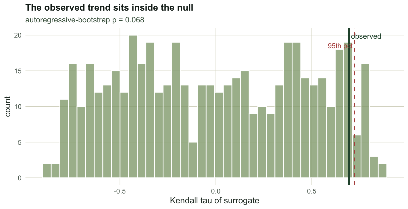
Here is the uncomfortable result. The autoregressive-bootstrap null puts its 95th percentile at 0.72, above the observed 0.69. The p-value is 0.068; the phase-randomised surrogates give 0.080. Neither reaches significance at the conventional 0.05. A series we built to approach a fold, with a clean rise in autocorrelation, does not clear a stationary null. The reason is that the trend statistic itself has a broad null distribution: rolling-window estimates from overlapping windows are strongly autocorrelated, so they drift up or down by chance far more than independent points would.

Figure 1: Surrogate null distribution of the autocorrelation trend statistic (autoregressive bootstrap). The observed value sits inside the null, short of the 95th percentile: the rise is not significant against a stationary process with the same short-term structure.

Check two: how often does it cry wolf?

If the null distribution is that broad, a naive test will over-declare warnings. We simulate many stationary records, the grazing model held at a constant c = 2.0 on the vegetated branch, with no approaching fold, and apply two tests to each: the naive Kendall test, which treats the window estimates as independent, and the surrogate test from above.

sim_stat <- function(seed, cc = 2.0, n = 200, dt = 0.05, sigma = 0.30, x0 = 7.32){
  set.seed(seed); ns <- n/dt; x <- numeric(ns); x[1] <- x0
  for(i in 2:ns){ x[i] <- x[i-1] + f(x[i-1], cc)*dt + sigma*sqrt(dt)*rnorm(1)
    if(x[i] < 0.001) x[i] <- 0.001 }
  x[seq(1, ns, by = 1/dt)] }

M <- 300; nb <- 200; naive_rej <- 0; surro_rej <- 0; tau_null <- numeric(M)
for(m in 1:M){
  y <- sim_stat(5000 + m); rr <- gauss_detrend(y, 0.10*nb)
  a <- roll_ar1(rr); to <- kt(a); tau_null[m] <- to
  pn <- cor.test(seq_along(a), a, method = "kendall")$p.value
  if(!is.na(pn) && pn < 0.05 && to > 0) naive_rej <- naive_rej + 1
  ps <- (1 + sum(arboot_taus(rr, 150, 9000 + m) >= to)) / 151
  if(ps < 0.05) surro_rej <- surro_rej + 1
}
naive_fp <- naive_rej/M; surro_fp <- surro_rej/M
sd_null <- sd(tau_null); frac_half <- mean(tau_null > 0.5)

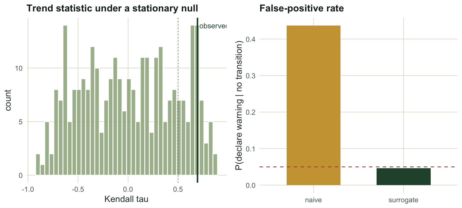
On stationary data with nothing approaching, the trend statistic has a standard deviation of 0.47 and exceeds 0.5 in 21 percent of runs by chance alone. The naive test declares a significant rising warning in 44 percent of these null records: it cries wolf almost half the time. The surrogate test brings the false-positive rate back to 5 percent, close to the nominal five. The lesson is blunt: a positive trend statistic assessed with an off-the-shelf significance test is nearly meaningless, and the observed 0.69 from a real approach is unremarkable against this spread.

Figure 2: Left: the trend statistic on stationary null records, centred at zero but very wide, with the observed value marked. Right: false-positive rate of the naive test versus the surrogate test; the dashed line is the nominal five percent.

Check three: necessary, not sufficient

Even a correct, significant rise is not proof of an approaching fold, and a fold can arrive with no rise at all. Two simulations make the point. First a false alarm: hold c constant, so there is no bifurcation anywhere, but let the process noise grow through the record. Nothing is destabilising, yet both indicators climb.

sim_risingnoise <- function(seed, cc = 2.0, n = 300, dt = 0.05, s0 = 0.12, s1 = 0.55, x0 = 7.32){
  set.seed(seed); ns <- n/dt; sv <- seq(s0, s1, length.out = ns); x <- numeric(ns); x[1] <- x0
  for(i in 2:ns){ x[i] <- x[i-1] + f(x[i-1], cc)*dt + sv[i-1]*sqrt(dt)*rnorm(1)
    if(x[i] < 0.001) x[i] <- 0.001 }
  x[seq(1, ns, by = 1/dt)] }
y_fa <- sim_risingnoise(seed = 4241); r_fa <- gauss_detrend(y_fa, 0.10*length(y_fa))
tau_var_fa <- kt(roll_var(r_fa)); tau_ar_fa <- kt(roll_ar1(r_fa))

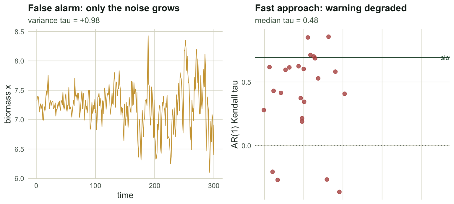
With no bifurcation in sight, the variance trend statistic is +0.98 and the autocorrelation one +0.72. Both fire, because the indicators respond to any change in the fluctuation structure, and a noisier environment is not an approaching fold.

Now the opposite failure: a real fold that arrives too fast to announce itself. Critical slowing needs a slow, quasi-static approach; when the driver is pushed quickly, the system tips through the fold before the indicators develop. We ramp the same driver over a much shorter record and look at the warning across thirty noise seeds.

sim_fast <- function(seed, T = 90, dt = 0.01, sigma = 0.30, c0 = 1.0, c1 = 2.95, x0 = 8.9){
  set.seed(seed); ns <- T/dt; cvec <- seq(c0, c1, length.out = ns); x <- numeric(ns); x[1] <- x0
  for(i in 2:ns){ x[i] <- x[i-1] + f(x[i-1], cvec[i-1])*dt + sigma*sqrt(dt)*rnorm(1)
    if(x[i] < 0.001) x[i] <- 0.001 }
  keep <- seq(1, ns, by = 1/dt); data.frame(t = (keep-1)*dt, x = x[keep], c = cvec[keep]) }

tau_fast <- c()
for(sd in 1:30){ df <- sim_fast(sd); tp <- which(df$x < 3.5)[1]
  if(is.na(tp) || tp < 40) next; sg <- df$x[1:(tp-4)]; if(length(sg) < 50) next
  tau_fast <- c(tau_fast, kt(roll_ar1(gauss_detrend(sg, 0.10*length(sg))))) }
med_fast <- median(tau_fast); lo_fast <- min(tau_fast); hi_fast <- max(tau_fast)

df12 <- sim_fast(12); tp12 <- which(df12$x < 3.5)[1]; sg12 <- df12$x[1:(tp12-4)]
r12 <- gauss_detrend(sg12, 0.10*length(sg12)); tau12 <- kt(roll_ar1(r12))
p12 <- (1 + sum(arboot_taus(r12, 500, 88) >= tau12)) / 501

The fast approach gives a median trend statistic of 0.48, well below the slow-approach 0.69, and across seeds it ranges from -0.36 to +0.86: some runs give a negative statistic, no warning at all. A representative run has trend statistic 0.43 and a surrogate p-value of 0.25, not significant. The same fold, approached quickly, is missed.

Figure 3: Left: a false alarm, constant driver with growing noise, no bifurcation, yet rising variance. Right: warning strength across noise seeds for a fast approach to a real fold, most falling well short of the slow-approach value.

Using early warning signals honestly

None of this retires the method. Critical slowing is a real phenomenon, and on long, slowly-forced systems the indicators do carry information. The point is what to claim from them. Three habits follow from the checks above. Assess significance against surrogates, never against a naive test, because the naive false-positive rate here was nearly half. Report the sensitivity to detrending and window choice from the previous tutorial, since a warning that survives only one setting is a choice, not a signal. And remember the base rate. Boettiger and Hastings (2012) call the common error a prosecutor’s fallacy: studying only the systems that collapsed inflates the apparent skill, because the probability of a warning given a transition is not the probability of a transition given a warning. Early warning signals are a screening tool that narrows hypotheses. They are necessary evidence of instability, not sufficient proof of it, and they are best reported as a tested hypothesis rather than a forecast.

References

• Scheffer et al. 2009 Nature 461(7260):53-59 (10.1038/nature08227)
• Dakos et al. 2012 PLoS ONE 7(7):e41010 (10.1371/journal.pone.0041010)
• Boettiger and Hastings 2012 Proceedings of the Royal Society B 279(1748):4734-4739 (10.1098/rspb.2012.2085)
• Boettiger, Ross and Hastings 2013 Theoretical Ecology 6(3):255-264 (10.1007/s12080-013-0192-6)
• Dakos et al. 2015 Philosophical Transactions of the Royal Society B 370(1659):20130263 (10.1098/rstb.2013.0263)

Related tutorials

• Early warning signals and critical slowing
• Detrending and bandwidth choice in early warning signals
• Spatial early warning signals
• Checking a time series model