Spatial early warning signals

Spatial variance, Moran’s I and spatial skewness measured on a coupled grazing lattice approaching a fold in R, with base stats only, and their caveats.

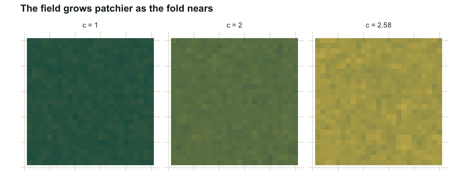
Corrected 14 October 2026: the caption of the field figure still called the field far from the fold smooth, a leftover of the earlier raw-biomass figure, and now says that the departures there are weak and fine-grained; the skewness paragraph and the caption of the indicator figure no longer read this single run as showing that the indicator fails on this lattice.

Corrected 1 October 2026: this post said its hand-coded Moran’s I used the same construction as the Moran’s I tutorial, which in fact uses spdep with weights on eight nearest neighbours. The field figure, which coloured raw biomass, mostly showed the falling mean; it now draws each snapshot as departures from its own mean, so the growing patchiness can be seen, and the skewness paragraph now says that its Kendall tau is computed on the signed values, so the magnitude, if anything, shrinks.

Critical slowing down has a spatial face. In a system where neighbouring patches interact, a slow recovery rate means a local perturbation spreads and lingers, so the correlation length grows. Snapshots of such a system, taken as a driver approaches a fold, should show rising spatial variance and rising spatial correlation even without any time series (Dakos et al. 2010; Kefi et al. 2014). A single well-sampled map can, in principle, carry the warning. This post builds a coupled grazing lattice, drives it towards collapse, and measures three proposed spatial indicators with base stats only.

A coupled grazing lattice

Each cell follows the same grazing dynamics as the temporal tutorial, with diffusive coupling to its four rook neighbours on a periodic grid, plus local noise. The grazing pressure c is held fixed within each snapshot and stepped up between snapshots.

r <- 1; K <- 10; h <- 1
f <- function(x, c) r*x*(1 - x/K) - c*x^2/(x^2 + h^2)

sim_spatial <- function(seed, L = 25, D = 0.30, sigma = 0.20, dt = 0.01,
                        c_snaps = c(1.0, 1.6, 2.0, 2.3, 2.5, 2.58), burn = 40, hold = 25){
  set.seed(seed)
  X <- matrix(8.9, L, L)
  neigh_mean <- function(M)                       # rook mean, periodic
    (M[c(L, 1:(L-1)), ] + M[c(2:L, 1), ] + M[, c(L, 1:(L-1))] + M[, c(2:L, 1)]) / 4
  step <- function(M, c){
    lap <- neigh_mean(M) - M
    M2 <- M + (f(M, c) + D*lap)*dt + sigma*sqrt(dt)*matrix(rnorm(L*L), L, L)
    M2[M2 < 0.001] <- 0.001; M2
  }
  snaps <- vector("list", length(c_snaps))
  for(s in seq_along(c_snaps)){
    cc <- c_snaps[s]
    for(i in 1:round(burn/dt)) X <- step(X, cc)   # relax towards a stationary field
    for(i in 1:round(hold/dt)) X <- step(X, cc)
    snaps[[s]] <- X
  }
  list(c = c_snaps, snaps = snaps, L = L)
}
sp <- sim_spatial(seed = 4240)

Three spatial indicators

Spatial variance is the variance across all cells. Spatial skewness is their third standardised moment. Spatial correlation we measure with Moran’s I, coded by hand with row-standardised rook weights on the periodic grid; the Moran’s I tutorial computes the same statistic with spdep, using row-standardised weights on each site’s eight nearest neighbours.

moran_grid <- function(M){
  L <- nrow(M); z <- as.vector(M) - mean(M); n <- L*L
  idx <- function(i, j) ((i-1) %% L)*L + ((j-1) %% L) + 1
  num <- 0
  for(i in 1:L) for(j in 1:L){
    nb <- c(z[idx(i-1, j)], z[idx(i+1, j)], z[idx(i, j-1)], z[idx(i, j+1)])
    num <- num + z[idx(i, j)] * sum(nb)/4          # row-standardised weights (1/4 each)
  }
  num / sum(z^2)                                    # (n / sum of weights) = 1 here
}
skew <- function(v){ v <- v - mean(v); mean(v^3) / (mean(v^2))^1.5 }

tab <- data.frame(
  c     = sp$c,
  mean  = sapply(sp$snaps, mean),
  s_var = sapply(sp$snaps, function(M) var(as.vector(M))),
  s_skew = sapply(sp$snaps, function(M) skew(as.vector(M))),
  moran = sapply(sp$snaps, moran_grid))

tau_var  <- cor(tab$c, tab$s_var,  method = "kendall")
tau_skew <- cor(tab$c, tab$s_skew, method = "kendall")
tau_moran <- cor(tab$c, tab$moran, method = "kendall")
var_fold <- tab$s_var[nrow(tab)] / tab$s_var[1]

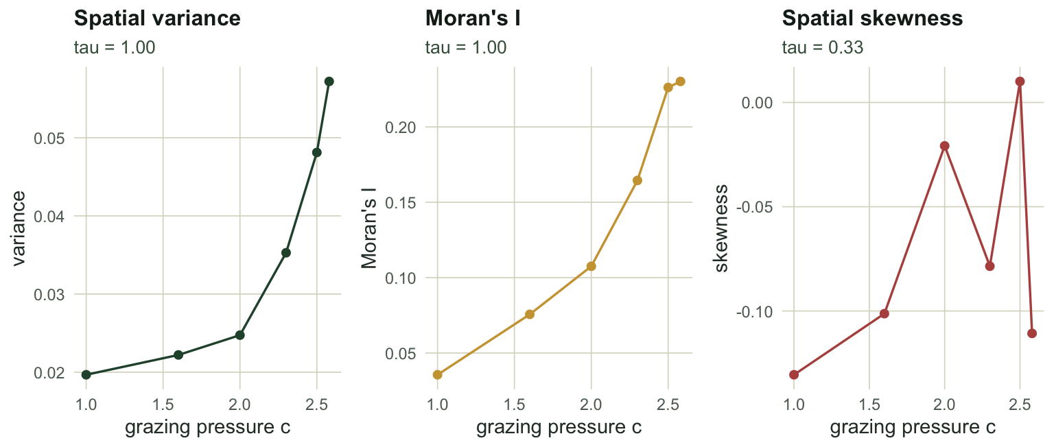
As the driver climbs from 1.0 to 2.58, the mean biomass falls from 8.89 to 5.23, tracking the sinking upper equilibrium. Spatial variance rises from 0.020 to 0.057, a 2.9-fold increase (Kendall tau = 1.00). Moran’s I moves from 0.036 to 0.230 (Kendall tau = 1.00). These are the spatial analogue of rising variance and rising lag-1 autocorrelation in time.

Figure 1: Biomass fields at three driver values, each drawn as departures from its own mean so that the colour shows patchiness rather than the falling mean. Far from the fold the departures are weak and fine-grained; approaching it, stronger correlated patches of high and low biomass emerge as the mean sinks.

Figure 2: The three spatial indicators against the driver. In this run, spatial skewness wanders with no clear trend.

The skewness caveat, and a deeper one

Spatial skewness is supposed to rise in magnitude near a fold, as the field starts to feel the lower state. Here it does not cooperate: its Kendall tau, computed on the signed values, is 0.33; as those values are mostly negative, the magnitude if anything shrinks, and it wanders between snapshots with no clear direction. A single snapshot is a noisy estimator of a third moment, and one realisation is not enough to pin it down, so this run may be an unlucky draw rather than a verdict on the indicator. This is worth stating plainly: an indicator can fail to show its expected trend in the one realisation you have, and reporting only the ones that rose would be the same selection error the checking tutorial warns about.

The deeper caveat applies to spatial variance and Moran’s I as well. Spatial variance and correlation rise for reasons other than an approaching fold. Self-organised vegetation patterns, environmental gradients, dispersal limitation, and measurement grain all raise spatial correlation without any loss of resilience. A patchy map is consistent with an approaching transition, but it is equally consistent with a landscape that is simply patchy. Spatial early warning signals narrow the hypotheses; they do not confirm one. The tools that turn a rising indicator into a tested claim are the subject of the final tutorial in this series.

References

• May 1977 Nature 269(5628):471-477 (10.1038/269471a0)
• Dakos et al. 2010 Theoretical Ecology 3:163-174 (10.1007/s12080-009-0060-6)
• Dai, Korolev and Gore 2013 Nature 496(7445):355-358 (10.1038/nature12071)
• Kefi et al. 2014 PLoS ONE 9(3):e92097 (10.1371/journal.pone.0092097)

Related tutorials

• Early warning signals and critical slowing
• Detrending and bandwidth in early warning signals
• Checking early warning signals
• Spatial autocorrelation and Moran’s I

Reproducibility

• Code last run: 2026-10-15
• R version 4.5.3 (2026-03-11), aarch64-apple-darwin20
• Packages: ggplot2 4.0.3