r <- 1; K <- 10; h <- 1
f <- function(x, c) r*x*(1 - x/K) - c*x^2/(x^2 + h^2)
sim_grazing <- function(seed, T = 600, dt = 0.01, sigma = 0.30,
                        c0 = 1.0, c1 = 2.72, x0 = 8.9){
  set.seed(seed); nstep <- T/dt; cvec <- seq(c0, c1, length.out = nstep)
  x <- numeric(nstep); x[1] <- x0
  for(i in 2:nstep){ x[i] <- x[i-1] + f(x[i-1], cvec[i-1])*dt + sigma*sqrt(dt)*rnorm(1)
    if(x[i] < 0.001) x[i] <- 0.001 }
  keep <- seq(1, nstep, by = 1/dt); data.frame(t = (keep-1)*dt, x = x[keep], c = cvec[keep])
}
d <- sim_grazing(seed = 4238)
tr_idx <- which(d$x < 3.5)[1]
seg <- d$x[1:(tr_idx - 10)]; n <- length(seg)Detrending and bandwidth in early warning signals
early warning signals
time series
R
resilience
ecology tutorial
The same collapsing series, four defensible detrending choices, and two sensitivity sweeps in R: how analyst decisions drive an early warning trend statistic.
Corrected 7 October 2026: the post said the two one-at-a-time sweeps show the full spread of the autocorrelation trend statistic an analyst could report; it now says they show how far each choice moves it alone, and that changing both at once reaches a wider range. The opening now says only that the indicators are usually not computed on the raw series.
Corrected 30 September 2026: the text said first-differencing removes any trend; it now says it removes a linear trend exactly and shrinks a slow curved one.
Early warning indicators are usually not computed on the raw series. They are computed on the residuals left after a slow trend is removed, because the trend itself inflates both variance and lag-1 autocorrelation. That detrending step, and the rolling-window width that follows it, are analyst choices with no objective setting. This post takes the collapsing grazing series from the critical slowing tutorial.
The same series as before
We regenerate the pre-transition record used earlier: a slow approach to a fold, sampled at unit intervals.
Four defensible ways to detrend
A Gaussian kernel smoother removes a local mean; its bandwidth sets how much wobble counts as trend. A small bandwidth follows the data closely and strips out slow structure; a large one leaves slow structure behind. First-differencing removes a linear trend exactly, and shrinks a slow curved one, without a bandwidth at all, but it reshapes the correlation structure. Centring only (no detrending) leaves the full trend in place. All four appear in the literature.
gauss_detrend <- function(y, bw){ tg <- seq_along(y)
  trend <- sapply(tg, function(i){ w <- dnorm(tg, i, bw); sum(w*y)/sum(w) }); y - trend }
roll_ar1 <- function(res, wf = 0.5){ win <- round(wf*length(res)); s <- 1:(length(res)-win+1)
  sapply(s, function(k){ w <- res[k:(k+win-1)]
    ar.ols(w, order.max = 1, aic = FALSE, demean = TRUE, intercept = FALSE)$ar[1] }) }
roll_var <- function(res, wf = 0.5){ win <- round(wf*length(res)); s <- 1:(length(res)-win+1)
  sapply(s, function(k) var(res[k:(k+win-1)])) }
kt <- function(v) cor(seq_along(v), v, method = "kendall")

res_raw  <- seg - mean(seg)             # no detrending
res_bw05 <- gauss_detrend(seg, 0.05*n)  # small bandwidth
res_bw25 <- gauss_detrend(seg, 0.25*n)  # large bandwidth
res_fd   <- diff(seg)                   # first difference

tau_ar_raw  <- kt(roll_ar1(res_raw));  tau_ar_bw05 <- kt(roll_ar1(res_bw05))
tau_ar_bw25 <- kt(roll_ar1(res_bw25)); tau_ar_fd   <- kt(roll_ar1(res_fd))
tau_var_raw  <- kt(roll_var(res_raw));  tau_var_bw05 <- kt(roll_var(res_bw05))
tau_var_bw25 <- kt(roll_var(res_bw25)); tau_var_fd   <- kt(roll_var(res_fd))
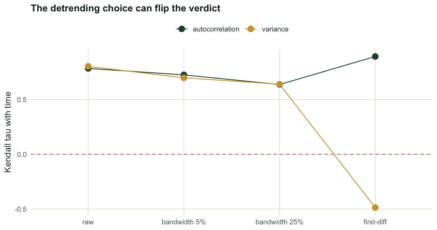
For the autocorrelation indicator every choice gives a positive trend: +0.78 (raw), +0.72 (bandwidth 5%), +0.64 (bandwidth 25%), +0.89 (first-difference). The autocorrelation warning survives the choice here.
Now the variance indicator. It reads +0.80 on the raw series, +0.70 and +0.64 under the two bandwidths, and -0.49 under first-differencing.
How far the choices reach
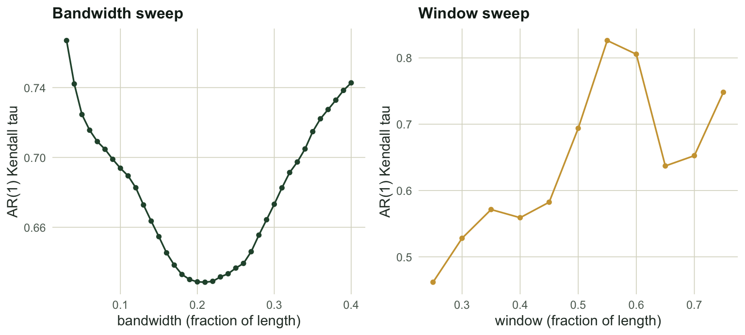
The two bandwidths above are just two points. Sweeping the Gaussian bandwidth across a plausible range, and separately sweeping the rolling-window width, shows how far each choice alone moves the autocorrelation trend statistic from this one series; an analyst free to change both at once could report a still wider range.
bws <- seq(0.03, 0.40, by = 0.01)
tau_bw <- sapply(bws, function(b) kt(roll_ar1(gauss_detrend(seg, b*n))))
res10 <- gauss_detrend(seg, 0.10*n)
wins <- seq(0.25, 0.75, by = 0.05)
tau_win <- sapply(wins, function(wf) kt(roll_ar1(res10, wf)))
bw_lo <- min(tau_bw); bw_hi <- max(tau_bw)
win_lo <- min(tau_win); win_hi <- max(tau_win)
win_at_hi <- wins[which.max(tau_win)]
The bandwidth choice alone moves the autocorrelation trend statistic across 0.63 to 0.77. The window width moves it from 0.46 to 0.83, the top of that range falling at a window of 55 per cent of the record. None of these settings is wrong. Each is a defensible default, and each yields a different number to put in a paper.
Reporting honestly
None of this means the indicators are useless. It means a single trend statistic, computed with one detrending method and one window width, is not a result on its own. Two habits help. Fix the analysis choices before looking at the outcome, so the bandwidth is not tuned towards the answer you hoped for. And report the sensitivity: show the trend statistic across a range of bandwidths and windows, not one number. On short ecological records, where there is little data to pin down the trend, this sensitivity is larger still. A warning that holds only for one bandwidth is not a warning; it is a choice. The checking tutorial adds the other half of the reckoning: whether a trend statistic, once chosen, is distinguishable from chance at all.
References
- Carpenter and Brock 2006 Ecology Letters 9(3):311-318 (10.1111/j.1461-0248.2005.00877.x)
- Dakos et al. 2012 PLoS ONE 7(7):e41010 (10.1371/journal.pone.0041010)
- Boettiger and Hastings 2012 Journal of the Royal Society Interface 9(75):2527-2539 (10.1098/rsif.2012.0125)
- Dakos et al. 2015 Philosophical Transactions of the Royal Society B 370(1659):20130263 (10.1098/rstb.2013.0263)