library(ggplot2)
library(patchwork)

te_paper  <- "#f5f4ee"
te_ink    <- "#16241d"
te_body   <- "#2c3a31"
te_forest <- "#275139"
te_rust   <- "#b5534e"
te_gold   <- "#c9b458"
te_line   <- "#dad9ca"

theme_datasheet <- function() {
  theme_minimal(base_size = 12) +
    theme(plot.background  = element_rect(fill = te_paper, colour = NA),
          panel.background = element_rect(fill = te_paper, colour = NA),
          panel.grid.major = element_line(colour = te_line, linewidth = 0.3),
          panel.grid.minor = element_blank(),
          text             = element_text(colour = te_body),
          plot.title       = element_text(colour = te_ink, face = "bold"),
          plot.subtitle    = element_text(colour = te_body),
          axis.text        = element_text(colour = te_body))
}
r_cols <- c(te_forest, te_gold, te_rust, te_ink)Red noise and extinction risk in a Ricker model
R
population dynamics
extinction
stochastic simulation
time series
ecology tutorial
At equal variance, red environmental noise raises extinction risk for an undercompensating Ricker population and lowers it for an overcompensating one, in R.
A natterjack toad pond on a dune slack fills in wet springs and dries out in dry ones. Wet years are not scattered at random through the record: they come in runs, because the water table carries one winter into the next and the weather itself has spells. Anyone who has kept a count for twenty years has seen three good years in a row and then four bad ones. The question for the viability assessment is simple to state. If the environment has memory, is the population in more danger or less than it would be if good and bad years arrived independently with the same spread?
The count-based population viability analysis on this site estimates the mean and variance of log growth from the counts and projects risk forward with each year an independent draw. The post on stochastic population growth draws good and bad years independently with fixed probabilities and shows what the variance does to the long-run growth rate. Mean time to extinction, exactly has no environment at all, only demographic chance. The post on wavelet significance and the red noise null uses a first order autoregressive process, but as a background against which to test for cycles, not as something a population lives through. None of them asks what the colour of the noise does to persistence, with its variance held fixed. That is the question here.
The folklore answer is that red noise, with positive autocorrelation, is dangerous because bad years cluster. Ripa and Lundberg 1996 showed that this depends on the population’s own dynamics, and Petchey, Gonzalez and Wilson 1997 found the sign of the effect set by the strength of density dependence. Heino, Ripa and Kaitala 2000 then pointed out that the answer also depends on what “the same variance” means. This post rebuilds both findings in base R, measures the size of each, and puts a measured quantity behind the explanation instead of a story.
A Ricker population with a coloured environment
The model is a Ricker map with two sources of chance. Each year the expected number of individuals next year is the current count times the Ricker growth factor, with an environmental deviation added to the log growth rate; the realised count is then a Poisson draw around that expectation, which is the demographic noise. A population is extinct when the integer count reaches zero, and zero is absorbing because a Poisson draw with mean zero is zero.
The growth parameter r sets the return dynamics. Linearised on the log scale around the carrying capacity, a deviation is multiplied by one minus r each year. Below r of one that multiplier is positive and the population creeps back towards the carrying capacity from one side, which is undercompensation. Above one it is negative, so a population above the carrying capacity is pushed below it the next year, which is overcompensation. At r of two the multiplier is minus one and the Ricker map is at its first period doubling.
The environmental deviation is a first order autoregressive process with lag one correlation rho. There are two ways to hold its variance fixed while rho changes, and they are not the same experiment. Under stationary scaling the variance of the deviation itself is fixed, so the innovation standard deviation is the target standard deviation times the square root of one minus rho squared. Under innovation scaling the yearly shock keeps a fixed standard deviation, and the variance of the deviation grows as one over one minus rho squared. The simulator takes the scaling as an argument, starts every replicate at the carrying capacity with the deviation drawn from its own stationary distribution, and runs all replicates as one vector.
k_cap     <- 30                                # carrying capacity
sd_env    <- 0.5                               # target noise standard deviation
n_years   <- 100                               # horizon
n_rep     <- 10000                             # replicates per cell, fixed in advance
n_mech    <- 2000                              # replicates per cell, skeleton check
rho_grid  <- c(-0.5, -0.25, 0, 0.25, 0.5, 0.65, 0.8)
r_grid    <- c(0.5, 1, 1.5, 2)
mcse_max  <- sqrt(0.25 / n_rep)

innov_sd <- function(rho, scaling) {
  ifelse(scaling == "stationary", sd_env * sqrt(1 - rho^2), sd_env)
}

sim_ricker <- function(n_rep, r, rho, scaling, k_cap = 30, n_years = 100,
                       threshold = 0, keep_log = FALSE) {
  s_inn <- innov_sd(rho, scaling)
  env   <- rnorm(n_rep, 0, s_inn / sqrt(1 - rho^2))
  n_now <- rep(k_cap, n_rep)
  gone  <- rep(FALSE, n_rep)
  log_n <- if (keep_log) matrix(NA_real_, n_years, n_rep) else NULL
  for (yr in seq_len(n_years)) {
    env   <- rho * env + rnorm(n_rep, 0, s_inn)
    n_now <- rpois(n_rep, n_now * exp(r * (1 - n_now / k_cap) + env))
    gone  <- gone | n_now <= threshold
    if (keep_log) log_n[yr, ] <- ifelse(n_now > 0, log(n_now / k_cap), NA)
  }
  list(extinct = mean(gone), log_n = log_n)
}
The scaling is the first thing a reviewer should check, so it is checked on the noise alone before any population is simulated.
ar_path <- function(n_steps, rho, scaling) {
  s_inn <- innov_sd(rho, scaling)
  env <- numeric(n_steps)
  env[1] <- rnorm(1, 0, s_inn / sqrt(1 - rho^2))
  shocks <- rnorm(n_steps, 0, s_inn)
  for (i in 2:n_steps) env[i] <- rho * env[i - 1] + shocks[i]
  env
}
n_check <- 200000
set.seed(4027)
noise_tab <- do.call(rbind, lapply(c("stationary", "innovation"), function(sc)
  do.call(rbind, lapply(c(-0.5, 0.8), function(rh) {
    env <- ar_path(n_check, rh, sc)
    data.frame(scaling = sc, rho = rh, sd_emp = sd(env),
               sd_target = innov_sd(rh, sc) / sqrt(1 - rh^2),
               lag1 = cor(env[-1], env[-n_check]))
  }))))
noise_gap <- max(abs(noise_tab$sd_emp / noise_tab$sd_target - 1))
lag_gap   <- max(abs(noise_tab$lag1 - noise_tab$rho))
sd_inn_08 <- noise_tab$sd_target[noise_tab$scaling == "innovation" & noise_tab$rho == 0.8]
noise_tab
scaling rho sd_emp sd_target lag1
1 stationary -0.5 0.5014611 0.5000000 -0.5015566
2 stationary 0.8 0.4994705 0.5000000 0.7994665
3 innovation -0.5 0.5788323 0.5773503 -0.5049706
4 innovation 0.8 0.8338099 0.8333333 0.8005844Over 200000 steps the empirical standard deviation of the deviation matches its target within 0.3 per cent in all four cases, and the lag one correlation matches rho within 0.005. Under stationary scaling the deviation has standard deviation 0.50 at every rho; under innovation scaling it is 0.833 at a rho of 0.8.
One noise series, two populations
Before counting extinctions it helps to watch what the two kinds of population do with the same weather. The chunk below drops the demographic draw and runs the deterministic Ricker skeleton on the log scale, fed with one shared sequence of standard normal shocks turned into white noise and into red noise with a rho of 0.8, both at the same stationary standard deviation.
n_show <- 60
set.seed(1908)
z_shared <- rnorm(n_show)
env_from <- function(z, rho) {
  env <- numeric(length(z)); env[1] <- sd_env * z[1]
  for (i in 2:length(z)) env[i] <- rho * env[i - 1] + sd_env * sqrt(1 - rho^2) * z[i]
  env
}
skeleton <- function(env, r) {
  x <- numeric(length(env)); x_prev <- 0
  for (i in seq_along(env)) { x[i] <- x_prev + r * (1 - exp(x_prev)) + env[i]; x_prev <- x[i] }
  x
}
path_tab <- do.call(rbind, lapply(c(0, 0.8), function(rh) {
  env <- env_from(z_shared, rh)
  do.call(rbind, lapply(c(0.5, 1.5), function(rr)
    data.frame(year = seq_len(n_show), rho = rh, r = rr, log_n = skeleton(env, rr))))
}))
path_tab$noise <- factor(ifelse(path_tab$rho == 0, "white noise", "red noise, rho 0.8"),
                         levels = c("white noise", "red noise, rho 0.8"))
path_tab$growth <- factor(sprintf("r = %.1f", path_tab$r))
path_min <- aggregate(log_n ~ rho + r, data = path_tab, FUN = min)
min_at <- function(rh, rr) path_min$log_n[path_min$rho == rh & path_min$r == rr]ggplot(path_tab, aes(year, log_n, colour = growth)) +
geom_hline(yintercept = 0, colour = te_body, linetype = "dashed", linewidth = 0.5) +
geom_line(linewidth = 0.8) +
facet_wrap(~ noise, ncol = 1) +
scale_colour_manual(values = c(te_forest, te_rust), name = NULL) +
labs(x = "year", y = "log(N / K)",
title = "Same shocks, different populations",
subtitle = "deterministic skeleton, no demographic draw") +
theme_datasheet() +
theme(legend.position = "bottom", strip.text = element_text(colour = te_ink, face = "bold"))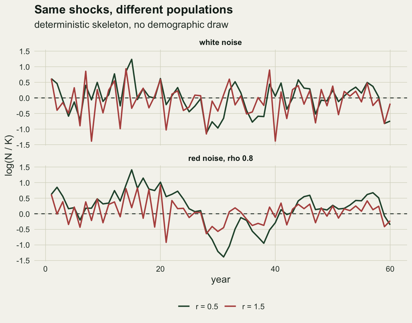
In white noise the lowest point of the undercompensating path is -1.13 on the log scale and of the overcompensating path -1.39. In red noise the order flips: -1.39 for r of 0.5 and -0.92 for r of 1.5. That is one series and proves nothing, but it shows the mechanism the rest of the post measures. An undercompensating population carries a run of bad years forward and keeps sliding; an overcompensating one reverses much of each year’s deviation the next year, and red noise hands it a deviation that is mostly last year’s again.
Extinction at fixed stationary variance
cells <- expand.grid(scaling = c("stationary", "innovation"), r = r_grid, rho = rho_grid,
                     stringsAsFactors = FALSE)
set.seed(5520)
cells$p_ext <- vapply(seq_len(nrow(cells)), function(i)
  sim_ricker(n_rep, cells$r[i], cells$rho[i], cells$scaling[i])$extinct, 0)
cells$mcse <- sqrt(cells$p_ext * (1 - cells$p_ext) / n_rep)
cells$growth <- factor(sprintf("r = %.1f", cells$r))
p_at <- function(rr, rh, sc = "stationary")
  cells$p_ext[cells$r == rr & cells$rho == rh & cells$scaling == sc]
stat_1 <- cells[cells$scaling == "stationary" & cells$r == 1, ]
r1_flat <- max(abs(stat_1$p_ext[stat_1$rho <= 0.25] - p_at(1, 0)))
Every cell uses 10000 replicates, a number fixed before the grid was run, so the Monte Carlo standard error of any extinction probability is at most 0.005.
At a stationary standard deviation of 0.5 and a carrying capacity of 30, the undercompensating population with r of 0.5 goes extinct within 100 years with probability 0.187 in white noise, 0.546 at a rho of 0.5 and 0.721 at 0.8. Negative autocorrelation, which alternates good and bad years, brings it down to 0.025. The overcompensating population with r of 1.5 runs the other way: 0.393 at a rho of minus 0.5, 0.259 in white noise and 0.049 at 0.8.
The population with r of one sits between them. Across rho from minus 0.5 to 0.25 its extinction probability moves by at most 0.011 from the white noise value of 0.040, but it rises to 0.216 at a rho of 0.8. At r of two, the edge of the stable range, extinction is 0.805 in white noise and falls steadily with reddening, from 0.922 at a rho of minus 0.5 to 0.326 at 0.8.
ggplot(cells[cells$scaling == "stationary", ], aes(rho, p_ext, colour = growth)) +
  geom_vline(xintercept = 0, colour = te_line, linewidth = 0.8) +
  geom_errorbar(aes(ymin = p_ext - 2 * mcse, ymax = p_ext + 2 * mcse),
                width = 0.03, linewidth = 0.4) +
  geom_line(linewidth = 0.9) + geom_point(size = 2.2) +
  scale_colour_manual(values = r_cols, name = NULL) +
  scale_y_continuous(limits = c(0, 1)) +
  labs(x = "lag one autocorrelation of the environment (rho)",
       y = "probability of extinction in 100 years",
       title = "Reddening helps some populations and hurts others",
       subtitle = "stationary noise sd fixed at 0.5, K = 30, bars: two Monte Carlo SE") +
  theme_datasheet() + theme(legend.position = "bottom")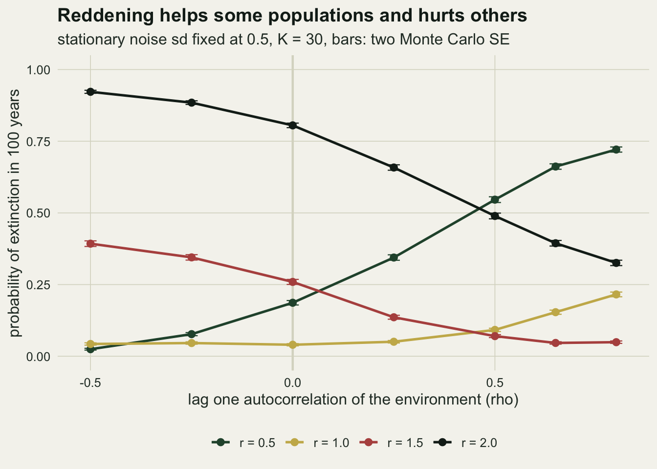
What the population does with the noise
The explanation offered above is that a population that returns from one side accumulates runs of deviations and one that overshoots cancels them. For r of 0.5 and 1.5 the multiplier one minus r has the same size and opposite signs, so the two return equally fast; what differs is the sign. That can be put in a number. Linearise the log abundance around the carrying capacity: the deviation next year is one minus r times this year’s deviation plus the environmental deviation. For a first order autoregressive input with stationary variance and correlation rho, the stationary variance of that linear filter has a closed form, the variance of the input times one plus lambda rho, divided by one minus lambda squared times one minus lambda rho, where lambda is one minus r.
With lambda positive the factor rises with rho; with lambda negative it falls; with lambda zero, at r of one, rho cancels out completely. That is the whole sign flip in one line, but it is a linear approximation, so it has to be checked against the nonlinear map. The check runs the same deterministic skeleton as the first figure, 2000 replicates per cell, and discards the first twenty years. The skeleton has no demographic draw, so no replicate is ever lost and the spread is not censored by extinction.
lin_sd <- function(r, rho, scaling) {
  lam <- 1 - r
  v_env <- innov_sd(rho, scaling)^2 / (1 - rho^2)
  sqrt(v_env * (1 + lam * rho) / ((1 - lam^2) * (1 - lam * rho)))
}
skeleton_spread <- function(n_rep, r, rho, scaling, n_years = 100, burn = 20) {
  s_inn <- innov_sd(rho, scaling)
  env <- rnorm(n_rep, 0, s_inn / sqrt(1 - rho^2))
  x_now <- rep(0, n_rep)
  x_mat <- matrix(NA_real_, n_years, n_rep)
  for (yr in seq_len(n_years)) {
    env <- rho * env + rnorm(n_rep, 0, s_inn)
    x_now <- x_now + r * (1 - exp(x_now)) + env
    x_mat[yr, ] <- x_now
  }
  kept <- x_mat[(burn + 1):n_years, ]
  c(sd_sim = sd(kept),
    lag1 = cor(as.vector(x_mat[burn:(n_years - 1), ]), as.vector(kept)))
}
burn <- 20
set.seed(7311)
mech <- t(vapply(seq_len(nrow(cells)), function(i)
  skeleton_spread(n_mech, cells$r[i], cells$rho[i], cells$scaling[i]), numeric(2)))
cells <- cbind(cells, as.data.frame(mech))
cells$sd_lin <- ifelse(cells$r < 2, lin_sd(cells$r, cells$rho, cells$scaling), NA)
m_at <- function(col, rr, rh, sc = "stationary")
  cells[[col]][cells$r == rr & cells$rho == rh & cells$scaling == sc]
stat_lin <- cells[cells$scaling == "stationary" & cells$r < 2, ]
stat_lin$ratio <- stat_lin$sd_sim / stat_lin$sd_lin
lin_ratio <- range(stat_lin$ratio)
worst_lin <- stat_lin[which.max(stat_lin$ratio), ]
For r of 0.5 the simulated standard deviation of log abundance rises from 0.456 at a rho of minus 0.5 to 0.611 in white noise and 1.675 at 0.8. For r of 1.5 it falls from 0.769 through 0.685 to 0.454. For r of one it runs from 0.530 to 0.652, where the linear formula holds it at 0.500.
The linear formula gets every direction right for r of 0.5 and 1.5 but not the size: across the stationary cells the simulated spread is between 1.02 and 1.90 times the linear value. The largest gap is at r of 0.5 and a rho of 0.80, where long excursions reach far enough from the carrying capacity for the curvature of the Ricker map to matter. On the log scale that curvature is lopsided: a population above the carrying capacity is pulled back by a term that grows exponentially, one below it by a term that can never exceed r. The same asymmetry is the most likely reason r of one responds to strong reddening when the linear filter says it should not.
The lag one autocorrelation of log abundance shows the tracking directly. At a rho of 0.8 it is 0.976 for r of 0.5, a population that follows the environment closely, and 0.275 for r of 1.5, whose own overshoot strips much of the persistence out of what it passes on.
mech_plot <- cells[cells$scaling == "stationary" & cells$r < 2, ]
ggplot(mech_plot, aes(rho, colour = growth)) +
  geom_line(aes(y = sd_lin), linetype = "dashed", linewidth = 0.7) +
  geom_line(aes(y = sd_sim), linewidth = 0.9) +
  geom_point(aes(y = sd_sim), size = 2.2) +
  scale_colour_manual(values = r_cols[1:3], name = NULL) +
  scale_y_continuous(limits = c(0, NA)) +
  labs(x = "lag one autocorrelation of the environment (rho)",
       y = "sd of log(N / K)",
       title = "The sign flip is already in the variance",
       subtitle = "solid with points: simulation, dashed: linear filter") +
  theme_datasheet() + theme(legend.position = "bottom")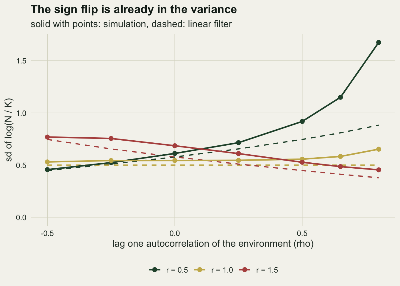
Holding the yearly shock fixed instead
Innovation scaling keeps the size of each year’s shock fixed and lets the variance of the environment grow with its autocorrelation. It answers a different question: not “what if the same spread of years were arranged differently” but “what if each year’s shock carried over more strongly”. Heino, Ripa and Kaitala 2000 showed that red and white noise can only be given the same variance at a chosen time scale, and that equally reasonable choices give qualitatively different answers; the stationary and innovation scalings here are two such choices.
inn_min_rho <- function(rr) {
  sub_cells <- cells[cells$scaling == "innovation" & cells$r == rr, ]
  sub_cells$rho[which.min(sub_cells$p_ext)]
}
inn_min_p <- function(rr) min(cells$p_ext[cells$scaling == "innovation" & cells$r == rr])
rank_rho <- cor(cells$sd_sim, cells$p_ext, method = "spearman")
rank_rho_r <- vapply(r_grid, function(rr) {
  sub_cells <- cells[cells$r == rr, ]
  cor(sub_cells$sd_sim, sub_cells$p_ext, method = "spearman")
}, 0)
fit_sd   <- glm(cbind(round(p_ext * n_rep), n_rep - round(p_ext * n_rep)) ~ log(sd_sim),
                family = binomial, data = cells)
fit_sd_r <- update(fit_sd, . ~ . + factor(r))
dev_drop <- 1 - deviance(fit_sd_r) / deviance(fit_sd)
r2_shift <- coef(fit_sd_r)[["factor(r)2"]]
At r of 0.5 innovation scaling makes reddening worse than it already was: extinction at a rho of 0.8 is 0.942 against 0.721 under stationary scaling. At r of 1.5 the benefit of reddening survives only up to a point. Extinction under innovation scaling is 0.636 at a rho of minus 0.5, reaches its lowest value on the grid, 0.173, at a rho of 0.25, and climbs back to 0.691 at 0.8, well above the white noise value of 0.258. The overcompensating population still cancels the colour, but it cannot cancel the extra variance that the innovation scaling adds as rho approaches one. At r of one the curve is also U shaped, with its minimum at a rho of 0.00.
If the variance of log abundance is what carries the effect, the extinction probabilities from both scalings and all four growth rates should line up when plotted against it. Across all 56 cells the Spearman rank correlation between the simulated standard deviation of log abundance and the extinction probability is 0.971. Within a single growth rate it is 0.987, 0.938, 0.991 and 0.956 for r of 0.5, 1, 1.5 and 2. The ranks agree, but the levels do not fully collapse: at the same spread the r of two cells go extinct more often than the r of 0.5 cells, visible as the black points above the green ones. In a binomial fit of extinction on log spread, adding growth rate as a factor removes 49 per cent of the residual deviance, and the r of two cells sit 0.86 higher on the logit scale than the r of 0.5 cells at the same spread.
scale_plot <- cells[cells$r < 2, ]
p_scale <- ggplot(scale_plot, aes(rho, p_ext, colour = growth, linetype = scaling)) +
  geom_line(linewidth = 0.8) + geom_point(size = 1.6) +
  scale_colour_manual(values = r_cols[1:3], name = NULL) +
  scale_linetype_manual(values = c(innovation = "dashed", stationary = "solid"), name = NULL) +
  scale_y_continuous(limits = c(0, 1)) +
  guides(colour = guide_legend(nrow = 1), linetype = guide_legend(nrow = 1)) +
  labs(x = "rho", y = "extinction probability, K = 30",
       title = "Two meanings of the same variance",
       subtitle = "solid: stationary scaling, dashed: innovation") +
  theme_datasheet() + theme(legend.position = "bottom", legend.box = "vertical")

p_collapse <- ggplot(cells, aes(sd_sim, p_ext, colour = growth, shape = scaling)) +
  geom_point(size = 2.4, stroke = 0.9) +
  scale_colour_manual(values = r_cols, name = NULL) +
  scale_shape_manual(values = c(innovation = 1, stationary = 16), name = NULL) +
  scale_x_log10() +
  scale_y_continuous(limits = c(0, 1)) +
  guides(colour = guide_legend(nrow = 1), shape = guide_legend(nrow = 1)) +
  labs(x = "sd of log(N / K), skeleton (log scale)",
       y = "extinction probability, K = 30",
       title = "One spread orders the cells",
       subtitle = "all cells, both scalings") +
  theme_datasheet() + theme(legend.position = "bottom", legend.box = "vertical")

p_scale + p_collapse + plot_annotation(theme = theme_datasheet())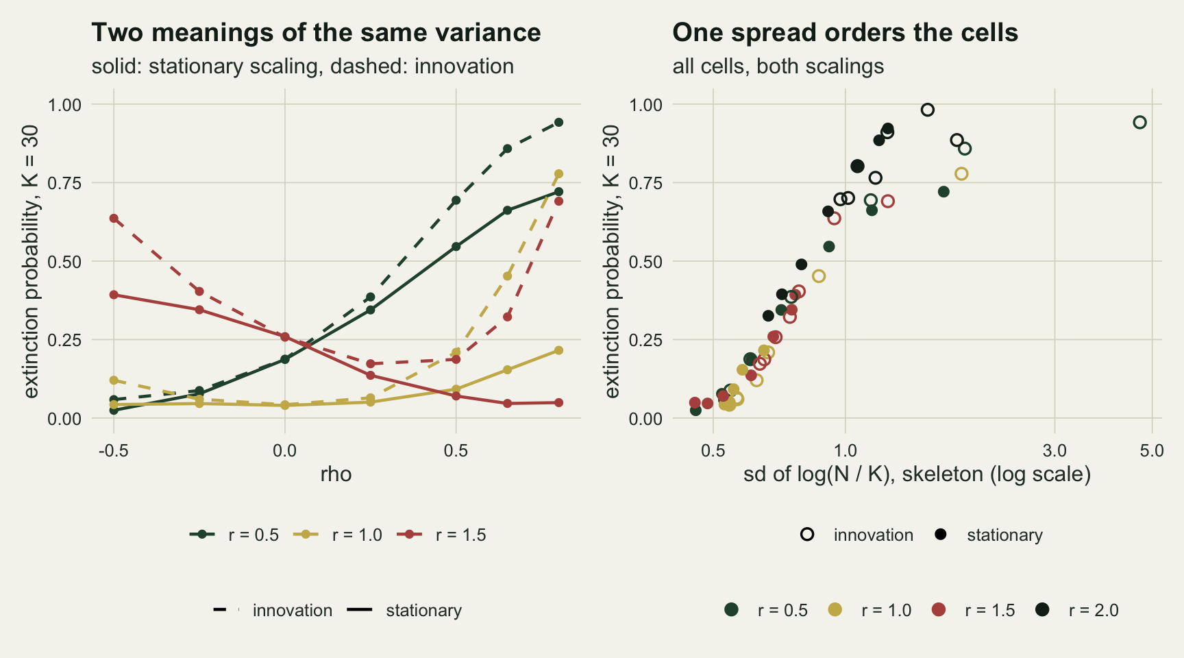
Carrying capacity and the extinction threshold
Two design choices could be doing the work: the carrying capacity of 30 and the definition of extinction as a count of zero. A Poisson population this small is exposed to demographic chance, and many assessments use a quasi-extinction threshold instead. The sign test below repeats the white noise and the rho 0.8 cells at three carrying capacities, with extinction defined either as zero or as falling below five individuals.
k_set <- c(15, 30, 60); quasi_thr <- 4
set.seed(6184)
rob <- expand.grid(k_cap = k_set, r = c(0.5, 1.5), threshold = c(0, quasi_thr))
rob$white <- NA_real_; rob$red <- NA_real_
for (i in seq_len(nrow(rob))) {
  rob$white[i] <- sim_ricker(n_rep, rob$r[i], 0, "stationary", k_cap = rob$k_cap[i],
                             threshold = rob$threshold[i])$extinct
  rob$red[i] <- sim_ricker(n_rep, rob$r[i], 0.8, "stationary", k_cap = rob$k_cap[i],
                           threshold = rob$threshold[i])$extinct
}
rob$shift <- rob$red - rob$white
expect_sign <- ifelse(rob$r < 1, 1, -1)
n_sign_ok <- sum(sign(rob$shift) == expect_sign)
rb <- function(kk, rr, th, col) rob[[col]][rob$k_cap == kk & rob$r == rr & rob$threshold == th]
bad <- rob[sign(rob$shift) != expect_sign, ]
rob$z <- rob$shift / sqrt((rob$white * (1 - rob$white) + rob$red * (1 - rob$red)) / n_rep)
bad_z <- rob$z[sign(rob$shift) != expect_sign]
ceil <- rob[rob$white > 0.99, ]
ceil_15 <- ceil[ceil$r == 1.5, ]
rest <- rob[rob$white <= 0.99, ]
n_rest_ok <- sum(sign(rest$shift) == ifelse(rest$r < 1, 1, -1))
rob
k_cap r threshold white red shift z
1 15 0.5 0 0.6300 0.8864 0.2564 44.379058
2 30 0.5 0 0.1852 0.7228 0.5376 90.707713
3 60 0.5 0 0.0295 0.5416 0.5121 97.318170
4 15 1.5 0 0.6003 0.2294 -0.3709 -57.456211
5 30 1.5 0 0.2496 0.0548 -0.1948 -39.838417
6 60 1.5 0 0.1106 0.0148 -0.0958 -28.505265
7 15 0.5 4 0.9989 0.9942 -0.0047 -5.672478
8 30 0.5 4 0.7569 0.9275 0.1706 34.035280
9 60 0.5 4 0.1928 0.7719 0.5791 100.549931
10 15 1.5 4 1.0000 0.9813 -0.0187 -13.804475
11 30 1.5 4 0.9250 0.3824 -0.5426 -98.161690
12 60 1.5 4 0.5395 0.0883 -0.4512 -78.669947The sign of the reddening effect is the expected one, up for r of 0.5 and down for r of 1.5, in 11 of the 12 combinations, but that count hides a reversal. The ceiling cases, the 2 combinations with a white noise risk above 0.99, are both at a carrying capacity of 15 with the quasi-extinction threshold. There reddening lowers the risk for both growth rates. For r of 0.5 it goes from 0.9989 to 0.9942, a drop of 0.0047 with a z of -5.7 (shift over its Monte Carlo standard error): a real reversal of the expected sign, if a small one. For r of 1.5 it goes from 1.0000 to 0.9813 (z of -13.8), which counts as the expected sign but comes from the same ceiling, so it is no better evidence for the rule. Away from the ceiling the sign held in 10 of the 10 remaining combinations, and there the smallest z in absolute value is 28.5.
The size of the effect does depend on the carrying capacity. At a carrying capacity of 15 and extinction at zero, reddening raises the risk for r of 0.5 from 0.630 to 0.886; at 60 it raises it from 0.029 to 0.542. For r of 1.5 at 60 the risk goes from 0.111 to 0.015. With the quasi-extinction threshold at a carrying capacity of 30, the r of 1.5 population goes from 0.925 in white noise to 0.382 in red, and the r of 0.5 population from 0.757 to 0.927.
What to report
Report the autocorrelation of the environmental driver, not only its variance, and say which variance is held fixed when rho is varied. A projection that holds the stationary variance fixed and one that holds the yearly shock fixed are different scenarios, and at r of 1.5 they disagree about the sign of the effect at strong reddening: 0.049 against 0.691, both compared with a white noise value near 0.26. For a field reader the stationary scaling is usually the honest one, because the variance of a climate index or of observed log growth is what a monitoring series measures; the innovation variance is a model quantity.
Report the return dynamics next to the risk. The same reddening of the same variance moved the hundred year extinction probability from 0.187 to 0.721 for an undercompensating population and from 0.259 to 0.049 for an overcompensating one. A statement that red noise raises extinction risk, without an estimate of how the population returns from a deviation, has no sign.
When the viability model is a count-based one with independent years, as in the population viability analysis post, the fitted variance of log growth already contains whatever colour the environment had over the monitoring period, filtered through the population. The projection then assumes that filtered variance is independent from year to year. The lag one autocorrelation of the residual log growth rates is the first thing to look at before trusting it.
Honest limits
The noise acts on the growth parameter only. Forcing the carrying capacity instead changes the transfer from environment to abundance, and Petchey, Gonzalez and Wilson 1997 found the sign of the colour effect set by density dependence in their model; nothing here tests whether the r of one boundary moves under that alternative. Ruokolainen and colleagues 2009 review the different ways noise has been inserted into population models and why they disagree.
The model is unstructured. Real populations have stages, and in a Leslie or stage structured model the answer depends on which vital rate the environment drives and on the generation time, which the single r of a Ricker map stands in for crudely. That comparison is not made here.
Only one horizon, one starting condition and one noise standard deviation were run. Every replicate starts at the carrying capacity, and one hundred years at a carrying capacity of 30 is long enough that some cells have extinction probabilities near one, where differences are compressed. A larger noise standard deviation would push more cells towards that ceiling.
The spread of log abundance that lines the cells up was measured on the deterministic skeleton, where extinction does not censor it, and the extinction probabilities on the Poisson model at a carrying capacity of 30. The rank correlation says the two orderings agree; it does not say that spread is the only thing that matters. Persistence of the deviations does not explain the remaining gap either: the r of two cells, whose log abundance is far less persistent than that of the r of 0.5 cells, are the ones that sit higher at the same spread, so the source of the gap was not identified here.
The case r of two sits at the first period doubling of the Ricker map, where the linear filter has no stationary variance and its formula was not used. Above it the deterministic dynamics cycle and then become chaotic, and the idea of a single return rate no longer applies. At r of two itself the return is neutrally stable in the linear approximation, so the skeleton spread depends on the burn-in and the horizon, and the r of two points in the right panel are indicative only. The noise is Gaussian and first order autoregressive; long memory and skewed environmental shocks, such as rare catastrophic droughts, were not examined.
References
Ripa J, Lundberg P 1996 Proceedings of the Royal Society B 263(1377):1751-1753 (10.1098/rspb.1996.0256)
Petchey OL, Gonzalez A, Wilson HB 1997 Proceedings of the Royal Society B 264(1389):1841-1847 (10.1098/rspb.1997.0254)
Heino M, Ripa J, Kaitala V 2000 Ecography 23(2):177-184 (10.1034/j.1600-0587.2000.230203.x)
Ruokolainen L, Linden A, Kaitala V, Fowler MS 2009 Trends in Ecology and Evolution 24(10):555-563 (10.1016/j.tree.2009.04.009)