library(ggplot2)

te_pal <- list(forest = "#275139", green = "#2f8f63", sage = "#93a87f",
               clay = "#b5534e", gold = "#cda23f", line = "#dad9ca",
               ink = "#16241d", paper = "#f5f4ee")

theme_te <- function() {
  theme_minimal(base_size = 12) +
    theme(panel.grid.minor = element_blank(),
          panel.grid.major = element_line(colour = "#e7e6dc"),
          plot.background = element_rect(fill = "#f5f4ee", colour = NA),
          panel.background = element_rect(fill = "#f5f4ee", colour = NA),
          plot.title = element_text(face = "bold", colour = te_pal$ink),
          axis.title = element_text(colour = "#2c3a31"),
          legend.position = "bottom")
}Mean time to extinction, exactly
R
stochastic simulation
population models
extinction
ecology tutorial
An exact double sum gives the mean time to extinction of a birth-death population in base R, checked against Gillespie simulation and diffusion theory.
The pool below the third weir holds a population of stone loach that somebody has been counting every spring since the mill was decommissioned. There are usually between eight and fifteen fish in it. The stretch of stream above the weir is culverted and the stretch below runs through a car park, so nothing arrives and nothing leaves; the pool is a closed system with a hard ceiling set by the amount of gravel. The obvious question from the water company, who would like to know whether to bother with a fish pass, is how long the population will last on its own.
That question has an exact answer, and it surprised me the first time I saw it. If you are willing to model the pool as a birth-death process on the integers, with a birth rate and a death rate attached to each possible population size, then the expected time until the population hits zero is not something you have to simulate. It is a double sum over ratios of the birth and death rates, it has no free parameters beyond the rates themselves, and it fits on one screen of base R. No approximation, no burn-in, no Monte Carlo error.
The reason this matters is that population viability analysis almost never uses it. The standard count-based machinery works on the logarithm of abundance and treats the population as a continuous quantity diffusing towards a quasi-extinction threshold. That is a sensible thing to do when your data are counts with observation error and you have no idea what the individual birth and death rates are. But it is an approximation, and once you have the exact answer sitting next to it you can measure how good the approximation is instead of hoping.
This post writes down the exact formula and checks it against an event-driven simulation, so that you can see the agreement land inside the Monte Carlo noise. It measures how the exact answer scales with carrying capacity, which decides whether persistence times are estimable at all. And it puts the diffusion approximation alongside the exact answer across a range of carrying capacities and reports the ratio, which turns out not to behave the way I expected.
Two existing posts on this blog cover the diffusion side. Population viability analysis and extinction risk fits the Dennis count-based model to a time series and reads extinction probabilities off it, and Stochastic population growth in variable environments handles the case where the growth rate itself varies year to year. Both of those work on the log scale with a continuous approximation to a process that is really jumps between integers. This post works on the integers with no approximation at all, and the comparison between the two is the whole point of the exercise. The event-driven sampler used for checking is built from scratch in The Gillespie algorithm from scratch, and it is reused here in compact form.
A logistic birth-death model on the integers
The state of the population is a non-negative integer. From state \(n\) the population goes up by one at rate \(b_n\) and down by one at rate \(d_n\), and the waiting time to the next event is exponential with rate \(b_n + d_n\). State zero is absorbing: once the last fish dies nothing brings it back, which is the whole point of the model.
The rates have to encode density dependence or the population either grows without limit or declines to zero deterministically, and neither of those is interesting. The version used here puts the density dependence entirely in the death rate:
\[b_n = B\,n, \qquad d_n = D\,n + (B - D)\,\frac{n^2}{K}\]
with \(B > D\). Births are linear in population size, deaths are linear plus a quadratic crowding term. The arithmetic is arranged so that at \(n = K\) the two rates are exactly equal, which makes \(K\) the deterministic equilibrium. Below \(K\) births win and the population grows; above \(K\) deaths win and it shrinks. The stochastic version has no equilibrium at all, because the only absorbing state is zero, and it will get there eventually from any starting point.
birth_rate <- 1.0     # per capita birth rate, B
death_rate <- 0.5     # per capita death rate at low density, D
K_sim      <- 10      # carrying capacity used for every simulation in this post
n_rep      <- 450     # Gillespie replicates per starting state
t_census   <- 25      # time at which surviving replicates are censused

b_of <- function(n, K, d0 = death_rate) birth_rate * n
d_of <- function(n, K, d0 = death_rate) d0 * n + (birth_rate - d0) * n^2 / K

print(c(K = K_sim, replicates = n_rep, census_time = t_census))
K replicates census_time
10 450 25 print(round(c(B = birth_rate, D = death_rate,
birth_at_K = b_of(K_sim, K_sim), death_at_K = d_of(K_sim, K_sim),
birth_at_half_K = b_of(K_sim / 2, K_sim),
death_at_half_K = d_of(K_sim / 2, K_sim)), 4)) B D birth_at_K death_at_K birth_at_half_K
1.00 0.50 10.00 10.00 5.00
death_at_half_K
3.75 The check in that output is the pair at \(n = K\): birth rate 10 and death rate 10, equal to four decimal places because they are equal exactly. At half the carrying capacity the birth rate is 5 against a death rate of 3.75, so the population there is growing at a per capita rate of a quarter per unit time. That is a healthy population by any field standard, and it will still go extinct.
The carrying capacity is set to 10, which is small. That is deliberate and it is the main constraint on everything that follows. The mean time to extinction grows so fast with \(K\) that a simulation at a carrying capacity of a few hundred would never finish inside a sensible knit budget: most replicates would still be running when the sun went out. Keeping \(K\) in the tens means the simulations actually reach zero, so there is something to compare the formula against. Where no simulation is involved, and the arithmetic is exact and instant, the post pushes \(K\) much higher.
The units of time are whatever the rates are measured in. If \(B\) is one birth per individual per year then time is in years, and a mean extinction time of fifty means fifty years. Nothing in the formulae cares.
The exact answer: a backward recursion and a double sum
Write \(\tau_n\) for the expected time to reach zero starting from \(n\) individuals. Condition on the first event. From state \(n\) the process waits an exponential time with mean \(1/(b_n + d_n)\), then jumps up with probability \(b_n/(b_n + d_n)\) and down otherwise. That gives
\[(b_n + d_n)\,\tau_n = 1 + b_n\,\tau_{n+1} + d_n\,\tau_{n-1}\]
for every \(n \ge 1\), with \(\tau_0 = 0\). Rearranged in terms of the increments \(\delta_n = \tau_n - \tau_{n-1}\) this collapses to a single first-order recursion:
\[d_n\,\delta_n = 1 + b_n\,\delta_{n+1}\]
which is the form worth implementing. Truncate the chain at some large \(N\) by setting \(b_N = 0\), which forbids births out of the top state. Then \(\delta_N = 1/d_N\), and everything below follows by working downwards. The answer is \(\tau_n = \sum_{m \le n} \delta_m\).
tau_recursion <- function(K, N, d0 = death_rate) {
  n   <- 1:N
  lam <- b_of(n, K, d0)
  mu  <- d_of(n, K, d0)
  lam[N] <- 0                      # truncate: no birth out of the top state
  incr <- numeric(N)
  incr[N] <- 1 / mu[N]
  for (i in (N - 1):1) incr[i] <- (1 + lam[i] * incr[i + 1]) / mu[i]
  cumsum(incr)                     # element n is tau_n
}

N_cap  <- 12 * K_sim
tau_ex <- tau_recursion(K_sim, N_cap)

print(round(c(state_cap = N_cap, tau_1 = tau_ex[1], tau_2 = tau_ex[2],
              tau_5 = tau_ex[5], tau_10 = tau_ex[10]), 3))
state_cap tau_1 tau_2 tau_5 tau_10
120.000 22.674 34.145 46.764 51.393 print(c(low_cap = 6 * K_sim, mid_cap = 12 * K_sim, high_cap = 24 * K_sim)) low_cap mid_cap high_cap
60 120 240 print(round(c(tau_at_low_cap = tau_recursion(K_sim, 6 * K_sim)[K_sim],
tau_at_mid_cap = tau_recursion(K_sim, 12 * K_sim)[K_sim],
tau_at_high_cap = tau_recursion(K_sim, 24 * K_sim)[K_sim]), 6)) tau_at_low_cap tau_at_mid_cap tau_at_high_cap
51.39279 51.39279 51.39279 print(round(c(gain_1_to_5 = tau_ex[5] - tau_ex[1],
gain_5_to_10 = tau_ex[K_sim] - tau_ex[5],
gain_5_to_10_percent = 100 * (tau_ex[K_sim] / tau_ex[5] - 1),
ratio_10_to_1 = tau_ex[K_sim] / tau_ex[1]), 3)) gain_1_to_5 gain_5_to_10 gain_5_to_10_percent
24.089 4.629 9.899
ratio_10_to_1
2.267 The truncation is not a source of error here. Doubling the cap from 60 states to 120 and doubling again to 240 leaves the answer at 51.39279 in every case, identical to six decimal places. The reason is that the death rate grows quadratically while the birth rate grows linearly, so the chain has no real chance of wandering far above \(K\); the probability of ever visiting state 60 starting from 10 is small enough that it contributes nothing. For a model with weaker density dependence you would need to check this again rather than assume it.
The numbers themselves already say something. Starting from a single individual the expected time to extinction is 22.674, and starting from a full house of 10 it is 51.393, a ratio of 2.267. Adding nine individuals to a lone founder does not even manage to treble the expected persistence time, which is the first sign that the process spends most of its life in a fairly narrow band of population sizes and that where you start barely matters.
Now the closed form. Iterating the increment recursion instead of solving it numerically gives
\[\delta_m = \sum_{k \ge m} \frac{1}{d_k} \prod_{j=m}^{k-1} \frac{b_j}{d_j}, \qquad \tau_n = \sum_{m=1}^{n} \delta_m\]
which is the double sum over ratios of rate products. It is worth writing this out because the structure is informative: the inner product is the ratio of the product of birth rates to the product of death rates over a stretch of states, and it is that product, not any single rate, that controls how long the population lasts.
The obvious implementation computes the numerator and denominator products separately and divides. That fails on any problem of a useful size, and it fails silently, because both products overflow long before their ratio does. The fix is to accumulate the logarithm of the ratio, which stays small.
tau_doublesum <- function(K, N, d0 = death_rate) {
  n   <- 1:N
  lam <- b_of(n, K, d0)
  mu  <- d_of(n, K, d0)
  S   <- c(0, cumsum(log(lam) - log(mu)))   # S[j + 1] is the log ratio product up to j
  incr <- numeric(N)
  for (m in 1:N) {
    k <- m:N
    incr[m] <- sum(exp(S[k] - S[m] - log(mu[k])))
  }
  cumsum(incr)
}

tau_ds <- tau_doublesum(K_sim, N_cap)
agreement <- max(abs(tau_ds / tau_ex - 1))
print(signif(c(max_relative_difference = agreement), 3))
max_relative_difference
8.88e-16 lam_all <- b_of(1:N_cap, K_sim)
mu_all <- d_of(1:N_cap, K_sim)
S_all <- c(0, cumsum(log(lam_all) - log(mu_all)))
biggest <- max(vapply(1:N_cap, function(m)
max(S_all[m:N_cap] - S_all[m] - log(mu_all[m:N_cap])), numeric(1)))
lam_40 <- b_of(1:480, 40)
mu_40 <- d_of(1:480, 40)
S_40 <- c(0, cumsum(log(lam_40) - log(mu_40)))
biggest_40 <- max(vapply(1:480, function(m)
max(S_40[m:480] - S_40[m] - log(mu_40[m:480])), numeric(1)))
print(c(states_at_K40 = 480))states_at_K40
480 print(round(c(log_of_birth_product_K10 = sum(log(lam_all)),
log_of_birth_product_K40 = sum(log(lam_40)),
product_log_ratio = sum(log(lam_40)) / sum(log(lam_all)),
double_overflow_limit = log(.Machine$double.xmax)), 2))log_of_birth_product_K10 log_of_birth_product_K40 product_log_ratio
457.81 2487.42 5.43
double_overflow_limit
709.78 print(round(c(largest_exponent_used_K10 = biggest), 3))largest_exponent_used_K10
0.624 print(round(c(largest_exponent_used_K40 = biggest_40), 3))largest_exponent_used_K40
8.28 The two exact routes agree to 8.88e-16, which is machine precision. They are the same calculation written twice, so this is a test of my algebra rather than of the model, and that is exactly what it is for. If the recursion and the closed form had disagreed I would not have known which one to trust.
The overflow numbers are the reason for the logarithms. At a carrying capacity of 10 with 120 states, the product of all the birth rates has a logarithm of 457.81, and double precision runs out at 709.78. So the naive numerator is already two thirds of the way to the ceiling at this tiny problem size, and at a carrying capacity of forty with 480 states its logarithm is 2487.42, worse by a factor of 5.43 and far past the limit: there the naive product really does overflow to infinity. Meanwhile the largest exponent that the paired form actually evaluates is 0.624 at the small carrying capacity and 8.28 at the larger one. Pairing each birth rate with the death rate at the same state keeps the evaluated exponents in single figures rather than the hundreds or thousands the raw products reach, because the ratio \(b_j/d_j\) is near one across the whole range that matters. This is not a subtle numerical trick, but it is the difference between a formula that works and one that returns NaN.
Checking it against the Gillespie sampler
An exact formula that has never been checked against a simulation is a conjecture. The check is an event-driven sampler: from the current state, draw the waiting time as an exponential with rate \(b_n + d_n\), then flip a coin weighted by \(b_n/(b_n + d_n)\) to decide whether the event is a birth or a death. Repeat until the state is zero and return the elapsed time. That is the Gillespie algorithm with two reactions, and it is exact in the sense that it samples from the true law of the process with no time-step error.
gillespie_extinction <- function(n0, K, census_at) {
  n <- n0
  now <- 0
  census <- NA_real_
  while (n > 0) {
    lam <- b_of(n, K)
    mu  <- d_of(n, K)
    total <- lam + mu
    nxt <- now - log(runif(1)) / total          # exponential waiting time
    if (is.na(census) && census_at <= nxt) census <- n
    now <- nxt
    if (runif(1) < lam / total) n <- n + 1 else n <- n - 1
  }
  c(extinction_time = now, census_state = census)
}

set.seed(20260728)
start_states <- c(1, 2, 5, 10)
runs <- lapply(start_states, function(s)
  t(replicate(n_rep, gillespie_extinction(s, K_sim, t_census))))

check <- data.frame(
  n0        = start_states,
  exact     = round(tau_ex[start_states], 3),
  simulated = round(sapply(runs, function(m) mean(m[, 1])), 3),
  mc_se     = round(sapply(runs, function(m) sd(m[, 1]) / sqrt(n_rep)), 3))
check$rel_error <- round(check$simulated / check$exact - 1, 4)
check$z         <- round((check$simulated - check$exact) / check$mc_se, 2)
print(check)
n0 exact simulated mc_se rel_error z
1 1 22.674 22.188 1.839 -0.0214 -0.26
2 2 34.145 32.324 2.032 -0.0533 -0.90
3 5 46.764 42.834 2.155 -0.0840 -1.82
4 10 51.393 51.147 2.285 -0.0048 -0.11print(round(c(worst_percent = 100 * min(check$rel_error),
best_percent = 100 * max(check$rel_error),
worst_shortfall_percent = -100 * min(check$rel_error),
worst_z = min(check$z), best_z = max(check$z)), 2)) worst_percent best_percent worst_shortfall_percent
-8.40 -0.48 8.40
worst_z best_z
-1.82 -0.11 Four starting states, 450 replicates each. The relative errors run from -8.40 to -0.48 per cent, and the standardised discrepancies, which are the differences divided by their own Monte Carlo standard errors, run from -1.82 to -0.11. Nothing is more than two standard errors from the exact value, which is what agreement looks like at this replicate count.
The relative error is the number people quote and it is the less informative of the two. At the starting state of 5 the simulated mean is 8.40 per cent below the exact value, which looks like a discrepancy until you notice that the Monte Carlo standard error there is 2.155 on a mean of 42.834, so the standardised difference is only -1.82. With 450 replicates from a distribution whose standard deviation is about as large as its mean, you cannot resolve anything finer than a few per cent, and that is the honest resolution of the check.
That is also the argument for having the exact formula at all. To pin the mean extinction time down to one per cent by simulation you would need roughly ten thousand replicates, and every one has to run to extinction. The recursion returns the same number for every starting state at once.
curve_dat <- data.frame(n0 = 1:K_sim, tau = tau_ex[1:K_sim], series = "exact double sum")
point_dat <- data.frame(n0 = start_states,
                        tau = check$simulated,
                        lo  = check$simulated - 2 * check$mc_se,
                        hi  = check$simulated + 2 * check$mc_se,
                        series = "Gillespie mean")

ggplot(curve_dat, aes(n0, tau)) +
  geom_line(aes(colour = series), linewidth = 1.1) +
  geom_errorbar(data = point_dat, aes(ymin = lo, ymax = hi, colour = series),
                width = 0.3, linewidth = 0.7) +
  geom_point(data = point_dat, aes(colour = series), size = 2.6) +
  scale_colour_manual(values = c("exact double sum" = te_pal$forest,
                                 "Gillespie mean" = te_pal$clay), name = NULL) +
  scale_x_continuous(breaks = 1:K_sim) +
  labs(title = "Exact formula against simulation",
       x = "starting population size", y = "mean time to extinction") +
  theme_te()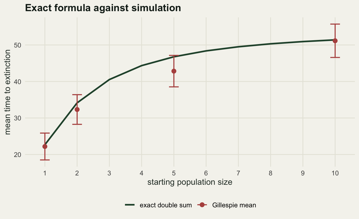
The shape of that curve is the biological content. It rises steeply from one individual to about four or five and then flattens almost completely. Going from 5 individuals to 10 buys you 4.629 extra units of expected persistence, a gain of 9.899 per cent, whereas going from one to 5 bought you 24.089. Once the population is anywhere near its ceiling, the expected time to extinction is essentially a property of the ceiling and not of the current count.
This is worth holding on to when reading a viability analysis that makes much of the current abundance. If the population is density-regulated and sitting near its equilibrium, whether the last census found eight animals or twelve tells you little about persistence.
Persistence time grows exponentially with carrying capacity
The flat top of that curve raises the obvious follow-up. If the starting count barely matters, what does? The answer is the carrying capacity, and the way it matters is the single most important quantitative fact about stochastic extinction.
Because the exact formula is instant, the scaling can be measured directly rather than argued for. Here it is evaluated across carrying capacities from six to forty at three different per capita death rates, holding the birth rate fixed. Changing the death rate changes both the population growth rate at low density and the strength of the crowding term, since the model keeps the equilibrium pinned at \(K\) by construction.
K_grid     <- seq(6, 40, by = 2)
death_grid <- c(0.35, 0.50, 0.65)

scaling <- do.call(rbind, lapply(death_grid, function(d0)
  data.frame(d0 = d0, K = K_grid,
             tau = sapply(K_grid, function(k) tau_recursion(k, 12 * k, d0)[k]))))

slope_of <- function(d0, kmin) {
  s <- scaling[scaling$d0 == d0 & scaling$K >= kmin, ]
  unname(coef(lm(log(s$tau) ~ s$K))[2])
}
analytic_exponent <- function(d0) (1 + d0 * log(d0) - d0) / (1 - d0)

scal_sum <- data.frame(
  death   = death_grid,
  slope   = round(sapply(death_grid, slope_of, kmin = min(K_grid)), 4),
  slope_upper = round(sapply(death_grid, slope_of, kmin = 24), 4),
  analytic = round(sapply(death_grid, analytic_exponent), 4),
  tau_K20 = signif(scaling$tau[scaling$K == 20], 5),
  tau_K40 = signif(scaling$tau[scaling$K == 40], 5))
print(scal_sum)
death slope slope_upper analytic tau_K20 tau_K40
1 0.35 0.3984 0.4147 0.4347 4584.00 17392000.0
2 0.50 0.2722 0.2850 0.3069 673.52 190400.0
3 0.65 0.1718 0.1760 0.2000 168.79 5484.3mid <- scaling[scaling$d0 == 0.50, ]
print(round(c(fold_range_at_K20 = scal_sum$tau_K20[1] / scal_sum$tau_K20[3],
fold_range_at_K40 = scal_sum$tau_K40[1] / scal_sum$tau_K40[3],
fold_K10_to_K40_mid = mid$tau[mid$K == 40] / mid$tau[mid$K == 10]), 1)) fold_range_at_K20 fold_range_at_K40 fold_K10_to_K40_mid
27.2 3171.2 3704.8 print(round(c(tau_K10_mid = mid$tau[mid$K == 10]), 3))tau_K10_mid
51.393 print(round(c(tau_K40_mid = mid$tau[mid$K == 40])))tau_K40_mid
190399 print(round(c(slope_mid = slope_of(0.50, min(K_grid)),
slope_mid_upper = slope_of(0.50, 24),
analytic_mid = analytic_exponent(0.50),
death_rate_span = max(death_grid) - min(death_grid)), 4)) slope_mid slope_mid_upper analytic_mid death_rate_span
0.2722 0.2850 0.3069 0.3000 Fit a straight line to the logarithm of mean extinction time against carrying capacity and the slope is 0.2722 at the middle death rate. Restricted to the upper half of the range it is 0.2850, drifting up, because the relationship has a slowly varying prefactor on the exponential and the fitted slope only approaches its limit from below. That limit can be written down. For this model the exponent is the integral of \(\log(b/d)\) across the population range from zero to \(K\), which evaluates to 0.3069 at a death rate of 0.50, and the fitted slopes are climbing towards it.
The consequence is what people get wrong. Mean time to extinction is not proportional to carrying capacity, it is exponential in it. Doubling the carrying capacity does not double persistence, it squares it, up to the slowly varying prefactor: at the small capacities used here that prefactor makes the squaring an overshoot. At the middle death rate the exact mean goes from 51.393 at a carrying capacity of ten to 190399 at forty, a factor of 3704.8 for a fourfold change in capacity.
scaling$rate <- factor(sprintf("%.2f", scaling$d0))

ggplot(scaling, aes(K, tau, colour = rate)) +
  geom_line(linewidth = 1.05) +
  geom_point(size = 1.6) +
  scale_y_log10(breaks = 10^(1:7),
                labels = parse(text = paste0("10^", 1:7))) +
  scale_colour_manual(values = c("0.35" = te_pal$forest,
                                 "0.50" = te_pal$gold,
                                 "0.65" = te_pal$clay),
                      name = "per capita death rate") +
  labs(title = "Persistence is exponential in carrying capacity",
       x = "carrying capacity", y = "mean time to extinction") +
  theme_te()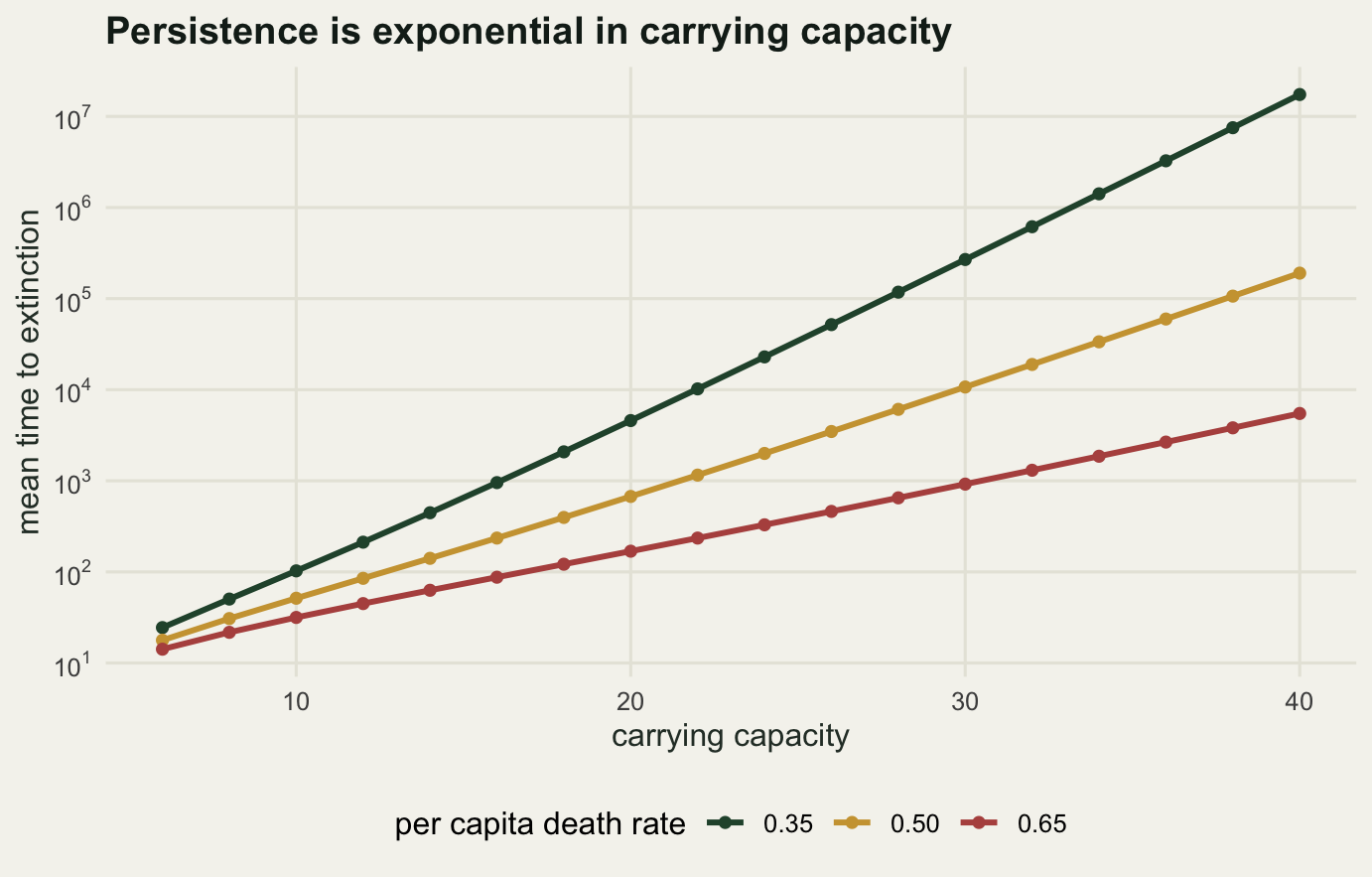
The three lines are straight on a logarithmic axis and they fan apart. That fanning is the practical result. At a carrying capacity of twenty, moving the per capita death rate from 0.35 to 0.65, a change of 0.3000 in a quantity you would struggle to measure to that precision from field data, moves the mean extinction time from 4584.00 down to 168.79, a factor of 27.2. At a carrying capacity of forty the same change in death rate moves it by a factor of 3171.2.
Read that again with a field notebook in mind. The demographic rates are the input; the persistence time is the output; and the map between them is exponential, with the carrying capacity in the exponent. A ten per cent error in an estimated death rate becomes a several-fold error in the predicted persistence time by the time the carrying capacity is a few dozen, and an order-of-magnitude error not far above that. Two studies of the same species that differ modestly in their estimated vital rates will produce persistence predictions that differ by a factor of a thousand, and both will look internally consistent.
This is the reason a persistence time is not something a short time series can estimate. It is not that the estimator is inefficient or that the confidence interval is wide. It is that the quantity being estimated is an exponential function of parameters whose uncertainty is irreducible at realistic sample sizes. Reporting a point estimate of mean time to extinction as a number of years, without the interval, is close to meaningless, and the interval will usually span several orders of magnitude if it is computed honestly.
The diffusion approximation, side by side
Count-based population viability analysis does not use the birth-death machinery. It uses a diffusion. The population size is treated as a continuous quantity, usually on the log scale, and the model keeps only the infinitesimal mean and variance of the change in \(\log N\) per unit time. For a birth-death process those follow from matching moments:
\[m(x) = \frac{b_n - d_n}{n} - \frac{b_n + d_n}{2n^2}, \qquad v(x) = \frac{b_n + d_n}{n^2}, \qquad n = e^{x}\]
where the second term in \(m\) is the correction that comes from working on the log scale. Given those two functions, the expected time for the diffusion to reach an absorbing boundary has a standard integral form built from the scale and speed densities, and it is the continuous analogue of the double sum above: an outer integral over the scale density of an inner integral of the speed density. The extinction boundary has to be placed somewhere, and the usual choice, which is the one used here, is a single individual.
tau_diffusion <- function(K, n0, d0 = death_rate, ngrid = 8001) {
  x <- seq(0, log(8 * K), length.out = ngrid)     # x = log n, boundary at n = 1
  h <- x[2] - x[1]
  n <- exp(x)
  bb <- b_of(n, K, d0)
  dd <- d_of(n, K, d0)
  m_inf <- (bb - dd) / n - (bb + dd) / (2 * n^2)
  v_inf <- (bb + dd) / n^2
  g <- 2 * m_inf / v_inf
  log_scale <- -c(0, cumsum((g[-1] + g[-ngrid]) / 2 * h))
  speed <- exp(-log(v_inf) - log_scale)
  inner <- c(rev(cumsum(rev((speed[-1] + speed[-ngrid]) / 2 * h))), 0)
  outer_int <- 2 * exp(log_scale) * inner
  approx(x, c(0, cumsum((outer_int[-1] + outer_int[-ngrid]) / 2 * h)), xout = log(n0))$y
}

K_diff <- c(seq(6, 40, by = 2), seq(50, 160, by = 10))
diff_tab <- data.frame(
  K         = K_diff,
  exact     = sapply(K_diff, function(k) tau_recursion(k, 12 * k)[k]),
  diffusion = sapply(K_diff, function(k) tau_diffusion(k, k)))
diff_tab$ratio <- diff_tab$diffusion / diff_tab$exact

print(signif(diff_tab[diff_tab$K %in% c(6, 10, 12, 20, 40, 80, 120, 160), ], 5))
K exact diffusion ratio
1 6 1.7782e+01 9.2857e+00 0.52220
3 10 5.1393e+01 2.8836e+01 0.56109
4 12 8.5039e+01 4.7903e+01 0.56331
8 20 6.7352e+02 3.6126e+02 0.53638
18 40 1.9040e+05 8.7519e+04 0.45966
22 80 2.7109e+10 9.8010e+09 0.36154
26 120 4.6512e+15 1.3449e+15 0.28916
30 160 8.5457e+20 1.9839e+20 0.23216print(round(c(exact_at_K10 = diff_tab$exact[diff_tab$K == 10],
diffusion_at_K10 = diff_tab$diffusion[diff_tab$K == 10],
ratio_at_K10 = diff_tab$ratio[diff_tab$K == 10]), 4)) exact_at_K10 diffusion_at_K10 ratio_at_K10
51.3928 28.8360 0.5611 grid_ratio <- tau_diffusion(160, 160, ngrid = 16001) /
tau_diffusion(160, 160, ngrid = 4001)
print(round(c(grid_refinement_ratio = grid_ratio), 6))grid_refinement_ratio
1.00002 The first thing the table says is that the diffusion is not close. At a carrying capacity of 10 it predicts 28.8360 against an exact 51.3928, a ratio of 0.5611. It is out by very nearly a factor of two, and it errs pessimistically: it says the population dies sooner than it really does.
The quadrature is not the problem. Refining the integration grid from four thousand points to sixteen thousand changes the answer at a carrying capacity of one hundred and sixty by a factor of 1.00002, a shift in the fifth significant figure. The gap between the diffusion and the exact answer is a property of the approximation, not of the arithmetic used to evaluate it.
The second thing the table says is the part I did not expect. The ratio does not improve as the carrying capacity grows.
best_at <- diff_tab$K[which.max(diff_tab$ratio)]
exponent_bd   <- 1 - log(2)
exponent_diff <- integrate(function(u)
  2 * (1 - death_rate) * (1 - u) / (1 + death_rate + (1 - death_rate) * u), 0, 1)$value
gap <- exponent_bd - exponent_diff
tail_fit <- coef(lm(log(ratio) ~ K, data = diff_tab[diff_tab$K >= 100, ]))

print(round(c(best_ratio = max(diff_tab$ratio), best_at_K = best_at,
              ratio_at_K6 = diff_tab$ratio[1],
              ratio_at_K160 = diff_tab$ratio[nrow(diff_tab)]), 4))
best_ratio best_at_K ratio_at_K6 ratio_at_K160
0.5633 12.0000 0.5222 0.2322 print(round(c(birth_death_exponent = exponent_bd,
diffusion_exponent = exponent_diff,
exponent_gap = gap,
fitted_tail_slope = unname(tail_fit[2])), 5))birth_death_exponent diffusion_exponent exponent_gap
0.30685 0.30146 0.00540
fitted_tail_slope
-0.00551 print(round(c(fitted_over_analytic = -unname(tail_fit[2]) / gap,
K_for_tenfold_error = log(10) / gap), 2))fitted_over_analytic K_for_tenfold_error
1.02 426.70 The ratio peaks at 0.5633 at a carrying capacity of 12, and falls away on both sides: 0.5222 at a carrying capacity of six, and 0.2322 at one hundred and sixty. So the approximation is worst where you might have expected it to be worst, at small population sizes, and also worst where you would have expected it to be best, at large ones.
The reason is exact and slightly beautiful. Both the exact process and its diffusion give a mean extinction time that grows exponentially in the carrying capacity, but with different exponents. For the birth-death chain the exponent is the integral of \(\log(b/d)\), which for this model is 0.30685. For the diffusion it is the integral of \(2(b-d)/(b+d)\), which is 0.30146. Those two integrands agree to second order in the difference between the rates and part company at third order, so the exponents differ by 0.00540. Fit a straight line to the logarithm of the ratio over the upper part of the range and the measured slope is -0.00551, which reproduces the analytic gap to a factor of 1.02.
A constant difference in the exponent means the ratio itself decays exponentially. The approximation is not off by a factor, it is off by a factor that grows without bound. Another ten-fold loss of accuracy takes a further 426.70 units of carrying capacity, a few hundred animals: entirely usual for a reserve population of a large vertebrate.
amp <- exp(mean(log(diff_tab$ratio[diff_tab$K >= 100]) +
                gap * diff_tab$K[diff_tab$K >= 100]))
asym <- data.frame(K = K_diff, ratio = amp * exp(-gap * K_diff),
                   series = "analytic decay")
meas <- data.frame(K = K_diff, ratio = diff_tab$ratio, series = "measured ratio")

ggplot(meas, aes(K, ratio)) +
  geom_hline(yintercept = 1, colour = te_pal$sage, linewidth = 0.7) +
  geom_line(data = asym, aes(colour = series), linewidth = 0.9, linetype = "dashed") +
  geom_line(aes(colour = series), linewidth = 1.05) +
  geom_point(aes(colour = series), size = 1.5) +
  scale_y_log10() +
  scale_colour_manual(values = c("measured ratio" = te_pal$forest,
                                 "analytic decay" = te_pal$clay), name = NULL) +
  guides(colour = guide_legend(override.aes = list(
    shape = c(NA, 16), linetype = c("dashed", "solid")))) +
  labs(title = "The diffusion gets worse, not better, with size",
       x = "carrying capacity", y = "diffusion / exact") +
  theme_te()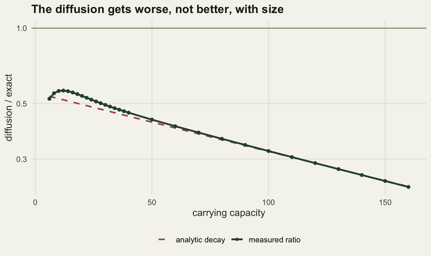
The horizontal reference line at the top of that panel is where a perfect approximation would sit. The measured curve never comes near it.
There is a second failure mode, and it is worse where it matters most. The diffusion has an absorbing boundary at one individual, which is a fudge: the real process is absorbed at zero, and zero is at minus infinity on the log scale. That fudge costs almost nothing when the population starts near its ceiling and everything when it starts near the boundary.
boundary <- data.frame(
  n0        = c(1, 2, 5, 10, 20),
  exact     = round(tau_recursion(20, 240)[c(1, 2, 5, 10, 20)], 2),
  diffusion = round(sapply(c(1, 2, 5, 10, 20), function(s) tau_diffusion(20, s)), 2))
boundary$ratio <- round(boundary$diffusion / boundary$exact, 4)
print(boundary)
n0 exact diffusion ratio
1 1 298.59 0.00 0.0000
2 2 454.35 147.53 0.3247
3 5 617.10 305.10 0.4944
4 10 662.87 350.57 0.5289
5 20 673.52 361.26 0.5364Starting from a single individual at a carrying capacity of twenty, the exact expected time to extinction is 298.59, because a lone individual has a decent chance of founding a population that then persists for a long time. The diffusion says 0, because the starting point is the absorbing boundary and the diffusion is absorbed immediately. From two individuals the ratio is 0.3247, and it only climbs back to 0.5364 once the population starts at its ceiling.
This is exactly the regime where a viability analysis is being asked to do real work: small founder groups, translocations, populations that have already crashed. The diffusion is comfortable in the middle of the distribution and unreliable at the edge, and the edge is where extinction happens.
None of this makes the diffusion useless. It uses far less information: only the mean and variance of the log growth rate, both estimable from a count series, whereas the exact formula needs \(b_n\) and \(d_n\) at every state, which you almost never have. Trading a factor of two for the ability to fit the model at all is often the right trade. The point is to know that the factor is there, that it grows with population size, and that it points the pessimistic way.
The quasi-stationary distribution, and what survivors look like
There is one more object in this model worth computing, and it explains something about simulation studies that is easy to get wrong.
Restrict the generator matrix of the process to the transient states, that is, drop the row and column for state zero. Call that sub-generator \(Q\). It is not a generator any more, because its rows do not sum to zero: probability leaks out of state one into extinction. The left eigenvector of \(Q\) belonging to the eigenvalue with the largest real part, normalised to sum to one, is the quasi-stationary distribution. It is the distribution of the population size conditional on not yet being extinct, in the limit of long time, and it is not the stationary distribution of the same process without absorption.
The eigenvalue itself is minus the decay rate. Call the decay rate \(\theta\). Once the process has settled into the quasi-stationary distribution it goes extinct at constant hazard \(\theta\), which means the remaining lifetime is exactly exponential with mean \(1/\theta\).
qsd_of <- function(K, N) {
  n   <- 1:N
  lam <- b_of(n, K)
  mu  <- d_of(n, K)
  lam[N] <- 0
  Q <- matrix(0, N, N)
  Q[cbind(n, n)] <- -(lam + mu)
  Q[cbind(1:(N - 1), 2:N)] <- lam[1:(N - 1)]
  Q[cbind(2:N, 1:(N - 1))] <- mu[2:N]
  ev <- eigen(t(Q))
  j  <- which.max(Re(ev$values))
  u  <- Re(ev$vectors[, j])
  list(u = u / sum(u), theta = -Re(ev$values[j]))
}

qs       <- qsd_of(K_sim, N_cap)
qsd_mean <- sum(qs$u * (1:N_cap))
qsd_sd   <- sqrt(sum(qs$u * (1:N_cap)^2) - qsd_mean^2)

print(round(c(theta = qs$theta, leak_check = qs$u[1] * d_of(1, K_sim)), 6))
theta leak_check
0.020988 0.020988 print(round(c(mean_life_from_qsd = 1 / qs$theta, exact_from_K = tau_ex[K_sim],
settling_gap = tau_ex[K_sim] - 1 / qs$theta,
qsd_mean = qsd_mean, qsd_sd = qsd_sd), 3))mean_life_from_qsd exact_from_K settling_gap qsd_mean
47.647 51.393 3.746 8.173
qsd_sd
4.285 print(c(qsd_mode = which.max(qs$u)))qsd_mode
7 print(round(c(qsd_shortfall_percent = 100 * (1 - qsd_mean / K_sim)), 1))qsd_shortfall_percent
18.3 The decay rate is 0.020988, so a population that has settled down has a mean remaining lifetime of 47.647. The exact mean starting from a full house of 10 is 51.393, which is longer by 3.746: that difference is the time the process spends sliding down from the ceiling into its quasi-stationary shape, and it is small because the slide is quick.
The consistency check in that output is worth pausing on. The rate at which probability leaks out of the transient states is the probability of being in state one times the death rate from state one, and that comes to 0.020988, identical to the decay rate 0.020988 obtained from the eigenvalue. Two independent routes to the same number is the only kind of check on an eigenvector calculation that is worth anything.
Now the part that matters for anybody who runs simulations. The quasi-stationary mean is 8.173, against a deterministic equilibrium of 10. The mode is at 7. Surviving populations sit systematically below the carrying capacity, by 18.3 per cent here, and the distribution has a standard deviation of 4.285, which is just over half its mean. That is not a transient, it is the stationary state of the conditioned process.
which_K    <- which(start_states == K_sim)
survivors  <- runs[[which_K]][, 2]
alive      <- !is.na(survivors)
emp_qsd    <- as.numeric(table(factor(survivors[alive], levels = 1:N_cap))) / sum(alive)
tv_dist    <- 0.5 * sum(abs(emp_qsd - qs$u))

print(c(replicates = n_rep, survivors = sum(alive)))
replicates survivors
450 282 print(round(c(survival_fraction = mean(alive),
predicted_fraction = exp(-qs$theta * t_census),
survivor_mean = mean(survivors[alive]), qsd_mean = qsd_mean,
total_variation_distance = tv_dist), 4)) survival_fraction predicted_fraction survivor_mean
0.6267 0.5917 8.2270
qsd_mean total_variation_distance
8.1729 0.0897 Of 450 replicates started at the carrying capacity, 282 were still alive at time 25, a fraction of 0.6267 against 0.5917 from the constant hazard alone: the excess is the settling period, during which the population sits above the quasi-stationary mean and is harder to kill. The survivors averaged 8.2270 individuals against a stationary mean of 8.1729, and the total variation distance between the simulated and the exact distribution is 0.0897, about as small as sampling error allows for 282 draws spread over a dozen states.
Here is the practical warning. Suppose you run a simulation study, discard the replicates that went extinct because they have nothing left to measure, and report the mean population size over the survivors. You have not measured the population. You have measured the quasi-stationary distribution, and it sits 18.3 per cent below the carrying capacity you put into the model. Conditioning on survival is a selection process, and it selects against the trajectories that wandered low, which are exactly the ones that drag the unconditioned mean down. Any summary computed over surviving replicates inherits that selection.
The extinction time is nearly exponential, but not quite
If the process reaches its quasi-stationary distribution quickly and then dies at constant hazard, the extinction time should be close to exponential. That has a sharp consequence: the coefficient of variation should be about one, and the median should sit at about 0.6931 of the mean, so that reporting the mean alone is a poor summary of a distribution in which more than half of the outcomes fall below it.
boot_stat <- function(x, f, B = 1500)
  sd(replicate(B, { i <- sample(length(x), length(x), TRUE); f(x[i]) }))

ext_from_K <- runs[[which_K]][, 1]
residual   <- ext_from_K[alive] - t_census
cv_f  <- function(z) sd(z) / mean(z)
med_f <- function(z) median(z) / mean(z)
delay <- tau_ex[K_sim] - 1 / qs$theta

set.seed(11002026)
cv_full_se  <- boot_stat(ext_from_K, cv_f)
cv_res_se   <- boot_stat(residual, cv_f)
med_full_se <- boot_stat(ext_from_K, med_f)
med_res_se  <- boot_stat(residual, med_f)

print(round(c(cv_from_K = cv_f(ext_from_K), cv_from_K_se = cv_full_se,
              cv_residual = cv_f(residual), cv_residual_se = cv_res_se,
              cv_of_an_exponential = 1), 4))
cv_from_K cv_from_K_se cv_residual
0.9476 0.0415 0.9868
cv_residual_se cv_of_an_exponential
0.0544 1.0000 print(round(c(median_ratio_from_K = med_f(ext_from_K),
median_ratio_from_K_se = med_full_se,
median_ratio_residual = med_f(residual),
median_ratio_residual_se = med_res_se,
median_ratio_of_an_exponential = log(2)), 4)) median_ratio_from_K median_ratio_from_K_se
0.6697 0.0354
median_ratio_residual median_ratio_residual_se
0.7406 0.0450
median_ratio_of_an_exponential
0.6931 print(round(c(settling_delay = delay,
predicted_cv = (1 / qs$theta) / tau_ex[K_sim],
predicted_median_ratio = (delay + log(2) / qs$theta) / tau_ex[K_sim],
residual_mean = mean(residual), one_over_theta = 1 / qs$theta), 4)) settling_delay predicted_cv predicted_median_ratio
3.7459 0.9271 0.7155
residual_mean one_over_theta
48.9460 47.6469 Starting from the carrying capacity, the coefficient of variation of the extinction time is 0.9476 with a bootstrap standard error of 0.0415. That is below one, and it is below one for a reason rather than by accident. The extinction time from a full population is the sum of two pieces: a short, nearly deterministic settling period while the population slides from the ceiling into its quasi-stationary shape, and then an exponential remaining lifetime. Adding a constant to an exponential leaves the standard deviation alone and increases the mean, so the coefficient of variation goes down. The settling delay here is 3.7459, and that decomposition predicts a coefficient of variation of 0.9271, which is within one bootstrap standard error of what was measured.
The clean test is to condition on survival and look at the remaining lifetime. Of the survivors at time 25, the mean remaining lifetime was 48.9460 against the theoretical 47.6469, and the coefficient of variation was 0.9868 with a bootstrap standard error of 0.0544. That is the exponential value of one to well inside the noise. Conditioning on having survived to a fixed time and then asking how much longer the population lasts gives back the same exponential distribution you started with, which is the memorylessness that the constant hazard implies.
The median ratios are noisier and they show the limit of the replicate count. Starting from the carrying capacity the measured median over mean is 0.6697 with a standard error of 0.0354, against an exponential value of 0.6931 and a predicted 0.7155. The two candidate values differ by less than one standard error, so 450 replicates cannot tell them apart. If you wanted to distinguish the shape of the extinction time distribution rather than just its mean, you would need several thousand replicates, and this is the same wall the mean ran into earlier.
show_to <- 20
panel_a <- data.frame(
  panel  = "Population size at the census (probability mass)",
  x      = rep(1:show_to, 2),
  y      = c(qs$u[1:show_to], emp_qsd[1:show_to]),
  series = rep(c("exact", "simulated"), each = show_to))

s_grid <- seq(0, 100, length.out = 41)
panel_b <- data.frame(
  panel  = "Time since the census (survival probability)",
  x      = rep(s_grid, 2),
  y      = c(exp(-qs$theta * s_grid),
             sapply(s_grid, function(v) mean(residual > v))),
  series = rep(c("exact", "simulated"), each = length(s_grid)))

both <- rbind(panel_a, panel_b)

ggplot(both, aes(x, y, colour = series)) +
  geom_line(linewidth = 0.9) +
  geom_point(size = 1.4) +
  facet_wrap(~ panel, scales = "free") +
  scale_colour_manual(values = c("exact" = te_pal$forest,
                                 "simulated" = te_pal$clay), name = NULL) +
  labs(title = "Survivors follow the quasi-stationary distribution",
       x = NULL, y = NULL) +
  theme_te()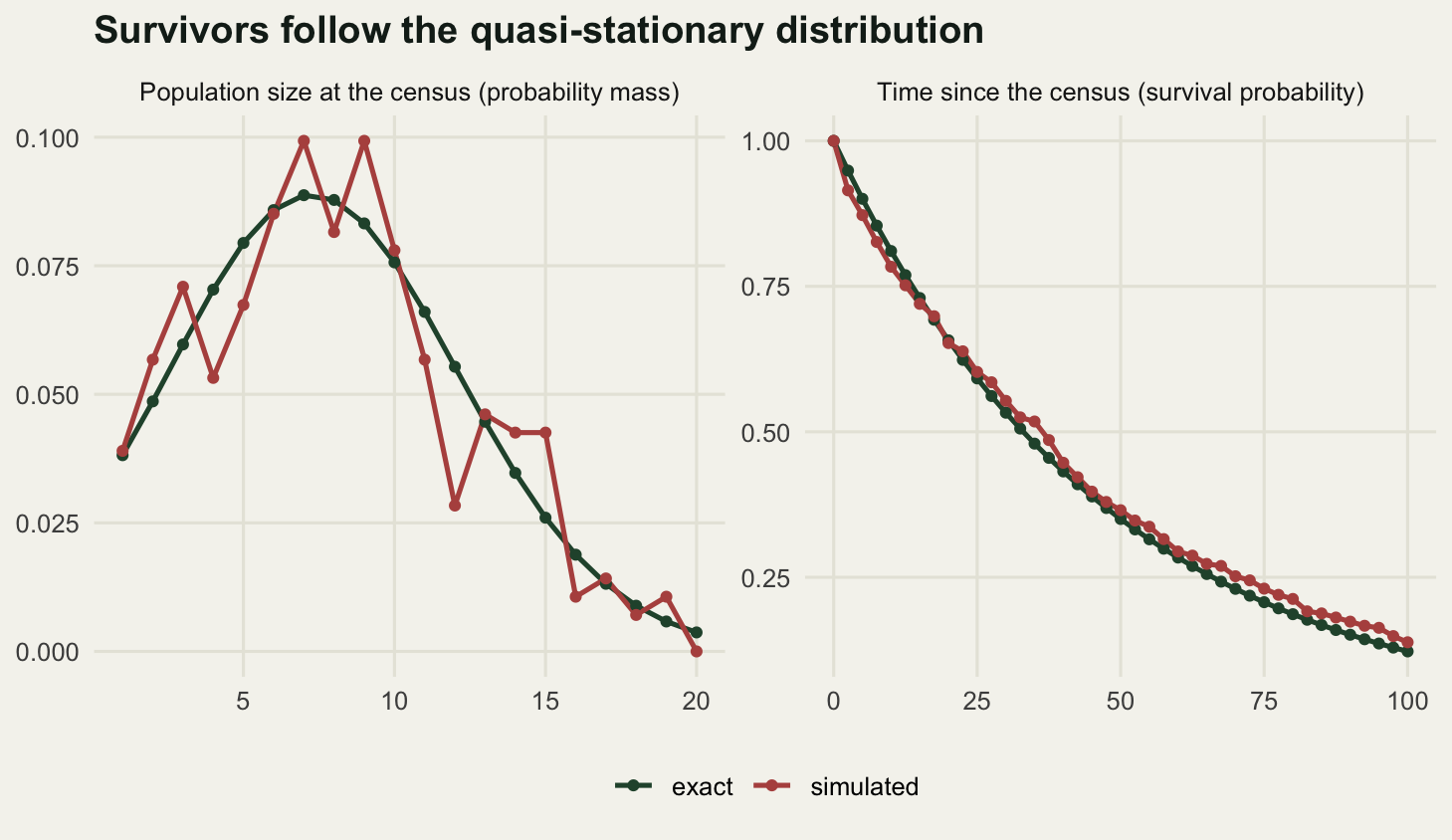
The right-hand panel is the memorylessness made visible. If extinction were a process that built up, with populations becoming progressively more fragile as time went on, that curve would start out flat and then fall away sharply, rather than dropping fastest at the very beginning as it does here. Instead the hazard is constant. A population that has lasted a long time is no more likely to go extinct in the next instant than one that has just settled down, because the only thing that matters is where it currently sits, and where it currently sits is drawn from the same quasi-stationary distribution either way.
That has an uncomfortable reading for anybody who has watched a small population persist for decades and concluded that it must be doing something right. Persistence is not evidence of health in a model like this one. Under a constant hazard, a fifth of the replicates last more than one and a half times the mean, and those look exactly like the short ones until they stop.
What to take away
The mean time to extinction of a birth-death population is a double sum you can evaluate in a few lines of base R, and it agrees with an exact event-driven simulation to within Monte Carlo error at every starting state tested. There is no reason to simulate this quantity if you know the rates. Write the increments as a backward recursion, accumulate the log ratio of birth to death rates rather than the two products separately, and check that the truncation cap does not move the answer.
The number that comes out grows exponentially with carrying capacity, with an exponent set by the integral of the log ratio of the rates. At the middle death rate used here the fitted slope over the upper part of the range was 0.2850 against an analytic 0.3069, and moving the per capita death rate from 0.35 to 0.65 at a carrying capacity of forty changed the persistence time by a factor of 3171.2. Persistence times are exponential functions of quantities you cannot measure precisely, which is why they should never be reported as bare point estimates.
The diffusion approximation that count-based viability analysis rests on underestimated the exact answer by about half at the small carrying capacities where the simulations here run, and the error grew with population size rather than shrinking: the ratio fell from a best value of 0.5633 at a carrying capacity of 12 to 0.2322 at one hundred and sixty, decaying at the analytic rate 0.00540 per unit of capacity. At the boundary it is worse still: starting from a single individual at a carrying capacity of twenty it returns 0 against an exact 298.59. Conditional on survival the population settles into a quasi-stationary distribution whose mean is 18.3 per cent below the carrying capacity, and the remaining lifetime from there is exponential, with a measured coefficient of variation of 0.9868 against the exponential value of one.
The honest limit is arithmetic, not biology. Everything above is exact for a model whose rates are known at every population size, and nobody knows that. Real rate estimates come from short records with wide intervals, often from a handful of years of counts with observation error folded in, and the exponential scaling turns those wide intervals into persistence predictions that span orders of magnitude. The exactness of the formula buys you a clean reference point against which to judge approximations; it does not buy you a number you can put in a management plan. Two further caveats sit alongside that one: the carrying capacity here is 10 because the simulations have to reach extinction inside a knit budget, so the simulation-based checks speak only for small populations, and the model has no environmental stochasticity at all, only demographic. Adding year-to-year variation in the rates changes the scaling from exponential in the carrying capacity to a power law, which is a different and generally much less optimistic story.
References
Gillespie DT 1977 The Journal of Physical Chemistry 81(25):2340-2361 (10.1021/j100540a008)
Dennis B, Munholland PL, Scott JM 1991 Ecological Monographs 61(2):115-143 (10.2307/1943004)
Lande R 1993 The American Naturalist 142(6):911-927 (10.1086/285580)
Doering CR, Sargsyan KV, Sander LM 2005 Multiscale Modeling and Simulation 3(2):283-299 (10.1137/030602800)
Ovaskainen O, Meerson B 2010 Trends in Ecology and Evolution 25(11):643-652 (10.1016/j.tree.2010.07.009)