library(ggplot2)

te_pal <- list(forest = "#275139", green = "#2f8f63", sage = "#93a87f",
               clay = "#b5534e", gold = "#cda23f", line = "#dad9ca",
               ink = "#16241d", paper = "#f5f4ee")

theme_te <- function() {
  theme_minimal(base_size = 12) +
    theme(panel.grid.minor = element_blank(),
          panel.grid.major = element_line(colour = "#e7e6dc"),
          plot.background = element_rect(fill = "#f5f4ee", colour = NA),
          panel.background = element_rect(fill = "#f5f4ee", colour = NA),
          plot.title = element_text(face = "bold", colour = te_pal$ink),
          axis.title = element_text(colour = "#2c3a31"),
          legend.position = "bottom")
}
The Gillespie algorithm from scratch
R
stochastic simulation
population models
ecology tutorial
Build the exact Gillespie stochastic simulation algorithm in base R, validate it against a Poisson stationary distribution, and measure what exactness costs.
A colleague counting great crested newts in a set of garden ponds once made a remark that stuck with me. Her spreadsheet had a column of integers, one per pond per visit, and every entry had been obtained by a person crouching in the dark with a torch. There was no version of her data in which a pond contained four and a half newts. The model she had been handed, on the other hand, was a differential equation whose solution passed smoothly through four and a half on its way from four to five, and it did so at every instant, in every pond, forever.
That mismatch is not pedantry. A pond with three newts and a pond with a smooth population density of three behave differently in exactly the situation an ecologist cares about most: near zero, where one animal more or less decides whether the local population persists. The differential equation cannot go extinct. It approaches zero and stays positive. The pond either has newts or it does not.
The fix is to simulate the thing that actually happens. Populations change by whole animals, one event at a time: a birth, a death, an immigrant arriving, an infection passing from one host to another. Between events nothing changes at all. If you are willing to say that the rate of each kind of event depends only on the current counts, then there is an algorithm that samples exactly from the process those rates define, with no time step, no discretisation and no approximation anywhere in it. It is about fifteen lines of base R. Daniel Gillespie published it for chemical kinetics in 1976 and 1977, and it has been carrying ecological models ever since.
This blog has used pieces of the machinery before without ever building the whole thing. The epidemic post Seasonality and recurrent epidemics runs a fixed-step tau leaping sampler in its critical community size section, which is an approximation to what we are about to build, and the coalescent posts draw exponential waiting times for a single kind of event. What has never appeared here is the exact algorithm as an object in its own right: the propensity vector, the exponential time to the next event of any type, the categorical draw for which type it was, and the argument for why that pair of draws is exact rather than merely good. That is what this post builds, and then it spends most of its length checking the result against mathematics that is known in closed form.
Everything here is base R plus ggplot2 for the pictures. The run sizes are deliberately modest, a few thousand short runs rather than a few hundred thousand, so the whole post knits in well under a minute on one core.
The two draws that make it exact
Write the state of the system as a vector of counts, \(x\). Give yourself a list of event types. Event \(j\) changes the state by a fixed integer vector \(\nu_j\) (one birth adds one to a count, one infection moves a host from susceptible to infected) and happens at a rate \(a_j(x)\) that depends on the current state and nothing else. That last clause is the whole modelling assumption. Ecologists usually call \(a_j\) a rate; the chemistry literature calls it a propensity, and the word is useful because it keeps you aware that the quantity is a rate per unit time for the whole system, not a per capita rate.
Now ask what happens next. Each event type \(j\), considered on its own with the state held fixed, fires after an exponential waiting time with rate \(a_j(x)\). The first thing to happen is the minimum of those independent exponentials. Two facts about exponentials do all the work. The minimum of independent exponential variables with rates \(a_1, a_2, \ldots\) is itself exponential with rate \(a_0 = \sum_j a_j\). And the probability that the minimum was achieved by type \(j\) is \(a_j / a_0\), independently of the value of the minimum.
So you do not have to draw one waiting time per event type. You draw the time to the next event of any type from an exponential with the total rate, then you draw which type it was from a categorical distribution with probabilities proportional to the individual rates. Update the state, update the clock, recompute the rates, repeat. Nothing is discretised and nothing is linearised. The sampler steps from one event to the next and lands exactly on the jump times of the process.
The exponential is not a modelling choice you make on top of the rates; it follows from them. If the rate of an event is a constant \(a\) for as long as the state does not change, then the probability of surviving a further interval without that event is the same whether you have already waited a long time or no time at all, and the only distribution with that property is the exponential. That is the whole content of the constant rate assumption, and it is also where the modelling risk sits. An animal whose death rate rises with its age, a host whose infectious period is roughly a fixed number of days rather than a random exponential one, a season that turns: none of those fit, and the sampler will happily produce exact draws from the wrong process if you give it one. Coming back to that is the closing point of the post.
There is one more thing to notice about the pair of draws, because it explains why nothing is lost by collapsing the event types into a total. The waiting time and the identity of the event are independent. Knowing that you waited a long time tells you nothing about which event finally fired, so the categorical draw does not have to be conditioned on the time you drew first. That independence is a property of competing exponentials specifically, and it is the reason this algorithm is two lines rather than a nested calculation.
Here is the direct method. The rates argument is a function from state to propensity vector, nu is a matrix with one row per event type, and the function records the whole path so we can plot it.
gillespie <- function(x0, nu, rates, t_max, cap = 20000L) {
  x <- x0; tnow <- 0; k <- 0L
  tvec <- numeric(cap + 1L); xmat <- matrix(0, cap + 1L, length(x0))
  tvec[1L] <- 0; xmat[1L, ] <- x0
  while (k < cap) {
    a <- rates(x); a0 <- sum(a)
    if (a0 <= 0) break
    tnow <- tnow - log(runif(1)) / a0
    if (tnow > t_max) break
    j <- which(cumsum(a) >= runif(1) * a0)[1L]
    x <- x + nu[j, ]; k <- k + 1L
    tvec[k + 1L] <- tnow; xmat[k + 1L, ] <- x
  }
  list(t = tvec[1:(k + 1L)], x = xmat[1:(k + 1L), , drop = FALSE], events = k)
}
Two lines deserve a second look. The waiting time is drawn as -log(runif(1)) / a0, which is inverse transform sampling for the exponential and is what rexp does internally; writing it out keeps the total rate a0 visible in the place where it belongs. The event type is drawn as which(cumsum(a) >= runif(1) * a0)[1L], which is the categorical draw done by walking up the cumulative rate vector until you pass a uniform point on the interval from zero to the total rate. That is the entire algorithm. There is no step size to choose, no tolerance, no solver.
The loop stops for one of three reasons: the clock has passed t_max, the total rate has fallen to zero (an absorbing state, which for a population model means extinction), or the event budget cap is exhausted. The budget exists only so that a badly parameterised model cannot run forever; every model below is checked to finish well inside it.
The first system to try is the simplest one that has a non-trivial answer. Immigrants arrive at a constant rate imm, independent of how many animals are already present, and each animal present dies at rate mu. Two event types, two lines of propensity. The deterministic version, \(dN/dt = \mathrm{imm} - \mu
N\), is a first-order linear equation whose solution from an empty patch is \(N(t) = (\mathrm{imm}/\mu)(1 - e^{-\mu t})\).
imm <- 2; mu <- 0.5; t_obs <- 16
nu_id <- matrix(c(1, -1), ncol = 1)
rates_id <- function(x) c(imm, mu * x[1])

set.seed(20260728)
one_run <- gillespie(c(0), nu_id, rates_id, t_obs, cap = 500L)
path <- data.frame(t = one_run$t, n = one_run$x[, 1])
path <- rbind(path, data.frame(t = t_obs, n = path$n[nrow(path)]))
det_curve <- data.frame(t = seq(0, t_obs, length.out = 400))
det_curve$n <- (imm / mu) * (1 - exp(-mu * det_curve$t))

empty_at <- one_run$t[one_run$x[, 1] == 0][-1]
print(round(c(immigration_rate = imm, per_capita_death_rate = mu,
              observation_time = t_obs,
              events_in_run = one_run$events,
              first_event_time = one_run$t[2],
              peak_count = max(one_run$x[, 1]),
              time_of_peak = one_run$t[which.max(one_run$x[, 1])],
              times_patch_empty = length(empty_at),
              first_empty = empty_at[1], second_empty = empty_at[2],
              deterministic_at_second_empty =
                (imm / mu) * (1 - exp(-mu * empty_at[2])),
              final_count = path$n[nrow(path)],
              deterministic_end = (imm / mu) * (1 - exp(-mu * t_obs))), 4))
immigration_rate per_capita_death_rate
2.0000 0.5000
observation_time events_in_run
16.0000 45.0000
first_event_time peak_count
0.5387 7.0000
time_of_peak times_patch_empty
4.7103 2.0000
first_empty second_empty
0.7651 10.6606
deterministic_at_second_empty final_count
3.9806 3.0000
deterministic_end
3.9987 ggplot() +
geom_step(data = path, aes(t, n, colour = "one exact realisation"),
linewidth = 0.7) +
geom_line(data = det_curve, aes(t, n, colour = "deterministic solution"),
linewidth = 1.1) +
scale_colour_manual(values = c("one exact realisation" = te_pal$green,
"deterministic solution" = te_pal$clay),
name = NULL) +
labs(title = "Whole animals, one event at a time",
x = "time", y = "count") +
theme_te()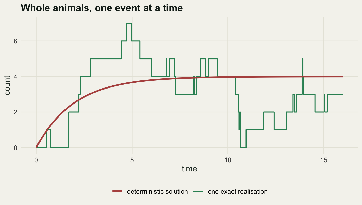
The realisation drawn here took 45 events to cross the 16 time units, and its first event landed at time 0.5387. It peaked at 7 animals at time 4.7103 and ended at 3, while the deterministic curve ends at 3.9987. Individually those numbers say nothing. What matters is the shape: the green path is flat between events and jumps by exactly one when an event happens, and it does not converge to anything, it keeps wandering. The clay curve is the average behaviour and no individual patch follows it.
One feature of the green path is worth pointing at directly, because it is the whole reason for the post. The count returned to zero twice, at time 0.7651 and again at time 10.6606. The patch was empty. Under immigration that is a temporary state and colonists arrive again, but in a model without immigration zero is absorbing and the run is over. The deterministic curve passes through 3.9806 animals at the second of those moments and has no way to express what happened.
Drawing the same law a different way
If the two-draw argument is right, then a sampler built the other way round has to give the same answer. The first-reaction method takes the description literally: draw one exponential waiting time per event type, find the smallest, advance the clock by it and fire that event. It throws away the other draws. It is wasteful, and Gillespie presented it mainly to motivate the direct method, but it is a genuinely different sampler and a good test.
gillespie_fr <- function(x0, nu, rates, t_max, cap = 20000L) {
  x <- x0; tnow <- 0; k <- 0L
  tvec <- numeric(cap + 1L); xmat <- matrix(0, cap + 1L, length(x0))
  tvec[1L] <- 0; xmat[1L, ] <- x0
  while (k < cap) {
    a <- rates(x)
    tau <- -log(runif(length(a))) / a          # Inf where a is zero
    j <- which.min(tau)
    if (!is.finite(tau[j])) break
    tnow <- tnow + tau[j]
    if (tnow > t_max) break
    x <- x + nu[j, ]; k <- k + 1L
    tvec[k + 1L] <- tnow; xmat[k + 1L, ] <- x
  }
  list(t = tvec[1:(k + 1L)], x = xmat[1:(k + 1L), , drop = FALSE], events = k)
}
To compare them we need a quantity with a distribution known in closed form. Take a pure death process: ten animals, each dying independently at rate mu_d, no births and no immigration. The time until the last one dies is the maximum of ten independent exponential lifetimes, so its distribution function is \(F(t) = (1 - e^{-\mu t})^{10}\) exactly. Its mean is \(\mu^{-1}\sum_{k=1}^{10} 1/k\) and its variance is \(\mu^{-2}\sum_{k=1}^{10} 1/k^2\), because the process spends an \(\mathrm{Exp}(k\mu)\) holding time in each state \(k\).
mu_d <- 0.4; n0_d <- 10; n_run_m <- 4000
nu_death <- matrix(-1, nrow = 1, ncol = 1)
rates_death <- function(x) c(mu_d * x[1])

ext_time <- function(fun, n_run) {
  vapply(seq_len(n_run), function(i) {
    r <- fun(c(n0_d), nu_death, rates_death, Inf, cap = 50L)
    r$t[length(r$t)]
  }, numeric(1))
}

set.seed(31082604)
e_dir <- ext_time(gillespie, n_run_m)
e_fr  <- ext_time(gillespie_fr, n_run_m)

cdf_ext <- function(z) (1 - exp(-mu_d * z))^n0_d
mean_exact <- sum(1 / (mu_d * (1:n0_d)))
sd_exact <- sqrt(sum(1 / (mu_d * (1:n0_d))^2))

kolm_p <- function(z) 2 * sum((-1)^(0:99) * exp(-2 * (1:100)^2 * z^2))
ks_one <- function(v, cdf) {
  n <- length(v); u <- sort(cdf(v))
  max(max((1:n) / n - u), max(u - (0:(n - 1)) / n))
}
ks_two <- function(v1, v2) {
  z <- sort(c(v1, v2)); max(abs(ecdf(v1)(z) - ecdf(v2)(z)))
}

d_dir <- ks_one(e_dir, cdf_ext)
d_fr <- ks_one(e_fr, cdf_ext)
d_two <- ks_two(e_dir, e_fr)

print(round(c(runs_per_method = n_run_m,
              mean_direct = mean(e_dir), mean_first = mean(e_fr),
              mean_exact = mean_exact,
              sd_direct = sd(e_dir), sd_first = sd(e_fr),
              sd_exact = sd_exact), 4))
runs_per_method mean_direct mean_first mean_exact sd_direct
4000.0000 7.2532 7.3083 7.3224 3.0970
sd_first sd_exact
3.0820 3.1122 print(round(c(D_direct_vs_exact = d_dir,
p_direct = kolm_p(sqrt(n_run_m) * d_dir),
D_first_vs_exact = d_fr,
p_first = kolm_p(sqrt(n_run_m) * d_fr),
D_direct_vs_first = d_two,
p_two_sample = kolm_p(sqrt(n_run_m / 2) * d_two)), 4))D_direct_vs_exact p_direct D_first_vs_exact p_first
0.0161 0.2486 0.0108 0.7433
D_direct_vs_first p_two_sample
0.0217 0.3004 With 4000 runs per method the direct sampler gives a mean extinction time of 7.2532 and the first-reaction sampler 7.3083, against the exact 7.3224. The standard deviations are 3.097 and 3.082 against the exact 3.1122. The Kolmogorov-Smirnov distance from the exact distribution function is 0.0161 for the direct method (p = 0.2486) and 0.0108 for first reaction (p = 0.7433). The two-sample distance between the samplers is 0.0217, p = 0.3004.
Three comparisons, none of them showing a discrepancy, and two of them against mathematics rather than against another simulation. That second point is the one to hold on to. A simulation checked only against another simulation can be wrong in the same way twice. The pure death process was chosen because its answer is a formula, and the formula does not care how you sampled.
The two samplers do not cost the same once a model has more than a couple of event types. The first-reaction method draws one uniform per event type per step and keeps only the smallest, so with two event types it draws two, the same as the direct method, but throws one of them away, and with twenty event types it draws twenty where the direct method still draws two. The waste is not just arithmetic: the draws it discards contain information, because an exponential that did not fire this step is still a valid partial waiting time for the next step once you rescale it. The next-reaction method exploits exactly that, keeping a priority queue of scheduled firing times and only recomputing the propensities that the last event actually changed. For a model with two or three event types, which covers most of what an ecologist writes down, the direct method is short enough and fast enough that the extra machinery is not worth it.
The p-values here are also a reminder about what a passed test means. Under the null the p-value is uniform on the unit interval, so a single value near 0.2486 or near one carries the same information: nothing detected at this sample size. A Kolmogorov-Smirnov test on 4000 draws would see a shift in the mean of roughly a few per cent. A bug that shifted the mean by half a per cent would sail straight through, which is why the next section compares a whole distribution cell by cell instead of testing it.
The calibration line: an exact stationary distribution
The immigration and death process has a property that makes it the best available test bed for an exact sampler. Started from an empty patch, the count at time \(t\) is exactly Poisson with mean \((\mathrm{imm}/\mu)(1 - e^{-\mu t})\), for every \(t\), not just in the limit. As \(t\) grows the mean approaches \(\mathrm{imm}/\mu\) and the stationary distribution is Poisson with that mean. There is nothing asymptotic about the claim and nothing to fit. If the sampler is exact, the histogram of final counts across independent runs is a Poisson sample, and any departure is Monte Carlo noise.
The comparison to make is not a test statistic but the distribution itself, cell by cell, against the noise you would expect if the sampler were perfect. That last part matters: a total variation distance of a hundredth means nothing until you know how big the total variation distance is between a perfect Poisson sample of the same size and the Poisson law it came from. So we simulate that reference too, by drawing Poisson samples of the same size with rpois and computing the same distance.
n_run_v <- 3000
set.seed(48151623)
fin <- numeric(n_run_v); ev_id <- numeric(n_run_v)
for (i in seq_len(n_run_v)) {
  r <- gillespie(c(0), nu_id, rates_id, t_obs, cap = 1000L)
  fin[i] <- r$x[nrow(r$x), 1]
  ev_id[i] <- r$events
}

lam <- imm / mu
lam_t <- lam * (1 - exp(-mu * t_obs))
k_max <- 13
obs_p <- tabulate(pmin(fin, k_max) + 1L, nbins = k_max + 1L) / n_run_v
exa_p <- dpois(0:k_max, lam)
exa_p[k_max + 1L] <- 1 - sum(exa_p[1:k_max])       # last cell is the upper tail
tvd <- 0.5 * sum(abs(obs_p - exa_p))
max_cell <- max(abs(obs_p - exa_p))

n_null <- 300
set.seed(90210777)
tv_null <- replicate(n_null, {
  z <- rpois(n_run_v, lam)
  0.5 * sum(abs(tabulate(pmin(z, k_max) + 1L, nbins = k_max + 1L) / n_run_v - exa_p))
})

print(round(c(runs = n_run_v, null_replicates = n_null,
              mean_events_per_run = mean(ev_id),
              exact_mean_at_t = lam_t, stationary_mean = lam,
              simulated_mean = mean(fin), simulated_variance = var(fin),
              total_variation = tvd, largest_cell_gap = max_cell,
              null_tv_mean = mean(tv_null),
              null_tv_q95 = unname(quantile(tv_null, 0.95))), 4))
runs null_replicates mean_events_per_run exact_mean_at_t
3000.0000 300.0000 59.6663 3.9987
stationary_mean simulated_mean simulated_variance total_variation
4.0000 4.0363 4.1537 0.0170
largest_cell_gap null_tv_mean null_tv_q95
0.0102 0.0216 0.0307 print(data.frame(n = 0:k_max,
simulated = round(obs_p, 4),
poisson = round(exa_p, 4),
difference = round(obs_p - exa_p, 4))) n simulated poisson difference
1 0 0.0200 0.0183 0.0017
2 1 0.0780 0.0733 0.0047
3 2 0.1363 0.1465 -0.0102
4 3 0.1927 0.1954 -0.0027
5 4 0.1930 0.1954 -0.0024
6 5 0.1557 0.1563 -0.0006
7 6 0.1040 0.1042 -0.0002
8 7 0.0637 0.0595 0.0041
9 8 0.0340 0.0298 0.0042
10 9 0.0143 0.0132 0.0011
11 10 0.0063 0.0053 0.0010
12 11 0.0010 0.0019 -0.0009
13 12 0.0007 0.0006 0.0000
14 13 0.0003 0.0003 0.0001The simulated mean is 4.0363 against the exact stationary 4, and against 3.9987, which is the exact mean at the observation time 16 and sits a thousandth below the stationary value. The simulated variance is 4.1537; for a Poisson distribution the variance equals the mean, and that is a second check the sampler was not asked to pass.
The distributional numbers are the point of the section. The total variation distance between the simulated distribution and the exact Poisson is 0.017, and the largest single cell discrepancy is 0.0102. Set against that, 300 perfect Poisson samples of the same size sit at a mean total variation distance of 0.0216 from the same exact law, with a ninety-fifth percentile of 0.0307. The sampler’s distance is smaller than the average distance achieved by a sample that came from the exact law by construction. There is no room left in that comparison for a systematic error: the discrepancy is pure sample size.
This is the chunk to copy when you write your own sampler for a model that nobody has tested. Strip your model back to a special case with a closed form, run the sampler on the special case, and compare the whole distribution against the formula with a noise reference computed the same way. A sampler that passes this on immigration and death, and passes the death process test above, has its exponential draws, its categorical draw and its bookkeeping all working.
pois_df <- data.frame(n = 0:k_max, simulated = obs_p, exact = exa_p)

ggplot(pois_df, aes(n)) +
  geom_col(aes(y = simulated, fill = "simulated"), width = 0.7) +
  geom_point(aes(y = exact, colour = "exact Poisson"), size = 2.4) +
  scale_fill_manual(values = c("simulated" = te_pal$green), name = NULL) +
  scale_colour_manual(values = c("exact Poisson" = te_pal$clay), name = NULL) +
  scale_x_continuous(breaks = 0:k_max) +
  labs(title = "The sampler against a closed form",
       x = "count at the observation time", y = "probability") +
  theme_te()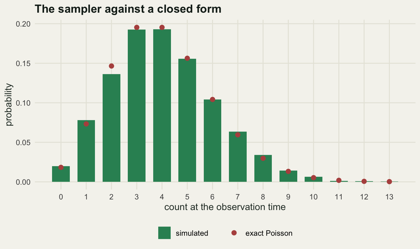
Nothing in the picture is meant to be surprising, and that is the use of it. When you later change the model and the bars stop sitting under the points, you know the change is in the model and not in the sampler.
A stochastic logistic population
Now a model with a nonlinearity. Births happen at rate \(bN\) and deaths at rate \(dN + (b - d)N^2/K\), so that the expected rate of change is \(rN(1 - N/K)\) with \(r = b - d\): the logistic equation, recovered exactly as the mean field limit. The extra deaths are the density dependence, and they are the only nonlinear term in the model.
The usual claim about this model is that the ensemble mean of the stochastic runs is not the deterministic solution, and the usual explanation is Jensen’s inequality: the death rate contains \(N^2\), and the expectation of \(N^2\) exceeds the square of the expectation by the variance, so the mean population feels more density dependence than the deterministic population does. That is true. The question this section actually answers is how much of the gap it accounts for, and the answer was not what I expected.
b_r <- 1; d_r <- 0.5; k_cap <- 40; n_start <- 4; t_end <- 20; n_run_l <- 500
nu_log <- matrix(c(1, -1), ncol = 1)
rates_log <- function(x) c(b_r * x[1], d_r * x[1] + (b_r - d_r) * x[1]^2 / k_cap)
t_grid <- seq(0, t_end, by = 0.25)

set.seed(70415529)
traj <- matrix(0, n_run_l, length(t_grid)); ev_log <- numeric(n_run_l)
for (i in seq_len(n_run_l)) {
  r <- gillespie(c(n_start), nu_log, rates_log, t_end, cap = 6000L)
  traj[i, ] <- r$x[findInterval(t_grid, r$t), 1]
  ev_log[i] <- r$events
}

r_growth <- b_r - d_r
det_n <- k_cap / (1 + (k_cap / n_start - 1) * exp(-r_growth * t_grid))
mean_all <- colMeans(traj)
alive <- traj[, ncol(traj)] > 0
mean_alive <- colMeans(traj[alive, , drop = FALSE])
gap_all <- det_n - mean_all
gap_alive <- det_n - mean_alive

late <- t_grid >= 14
pooled <- as.vector(traj[alive, late])
qs_mean <- mean(pooled); qs_var <- var(pooled)

last <- length(t_grid)
se_all <- sd(traj[, last]) / sqrt(n_run_l)
se_alive <- sd(traj[alive, last]) / sqrt(sum(alive))
early <- which(t_grid == 2)
gap_pct <- round(100 * gap_all[last] / det_n[last], 1)
gap_se_ratio <- round(gap_all[last] / se_all, 1)
pct_extinction <- round(100 * (1 - gap_alive[last] / gap_all[last]), 1)

print(round(c(runs = n_run_l, birth_coefficient = b_r, death_coefficient = d_r,
              carrying_capacity = k_cap, start_count = n_start,
              end_time = t_end, early_time = t_grid[early],
              mean_events_per_run = mean(ev_log),
              extinct_fraction = mean(!alive),
              extinct_percent = 100 * mean(!alive),
              extinct_se = sqrt(mean(!alive) * mean(alive) / n_run_l),
              linear_prediction = (d_r / b_r)^n_start), 4))
runs birth_coefficient death_coefficient carrying_capacity
500.0000 1.0000 0.5000 40.0000
start_count end_time early_time mean_events_per_run
4.0000 20.0000 2.0000 1021.4320
extinct_fraction extinct_percent extinct_se linear_prediction
0.0700 7.0000 0.0114 0.0625 print(round(c(deterministic_end = det_n[last],
ensemble_mean_end = mean_all[last], se_ensemble = se_all,
survivor_mean_end = mean_alive[last], se_survivors = se_alive,
sd_survivors_end = sd(traj[alive, last]),
gap_end = gap_all[last],
gap_percent_of_deterministic = gap_pct,
gap_in_standard_errors = gap_se_ratio,
gap_end_survivors = gap_alive[last],
share_from_extinction = 1 - gap_alive[last] / gap_all[last],
percent_from_extinction = pct_extinction,
largest_gap = max(gap_all),
time_of_largest_gap = t_grid[which.max(gap_all)],
gap_at_time_2 = gap_all[early],
se_at_time_2 = sd(traj[, early]) / sqrt(n_run_l)), 4)) deterministic_end ensemble_mean_end
39.9837 34.4880
se_ensemble survivor_mean_end
0.5702 37.0839
se_survivors sd_survivors_end
0.4104 8.8507
gap_end gap_percent_of_deterministic
5.4957 13.7000
gap_in_standard_errors gap_end_survivors
9.6000 2.8998
share_from_extinction percent_from_extinction
0.4723 47.2000
largest_gap time_of_largest_gap
6.8151 12.0000
gap_at_time_2 se_at_time_2
-0.3312 0.2699 print(round(c(quasi_stationary_mean = qs_mean,
quasi_stationary_variance = qs_var,
observed_deficit = k_cap - qs_mean,
moment_prediction = qs_var / qs_mean,
deficit_shortfall = (k_cap - qs_mean) - qs_var / qs_mean), 4)) quasi_stationary_mean quasi_stationary_variance observed_deficit
36.9593 85.0962 3.0407
moment_prediction deficit_shortfall
2.3024 0.7383 Start with the ensemble. At the end of the run the deterministic solution sits at 39.9837, effectively at the carrying capacity 40, while the mean over all 500 stochastic runs is 34.488 with a standard error of 0.5702. The gap is 5.4957 animals, about 13.7 per cent of the deterministic value and 9.6 standard errors wide, so it is a real feature and not sampling noise.
The gap is not constant over time. It reaches its largest value, 6.8151 animals, at time 12, on the upper shoulder of the deterministic curve, where most of its climb is done and the ensemble mean is still working its way up, and it then settles back to about 5.4957. Early on the sign is not even reliable: at time 2 the measured gap is -0.3312 animals against a standard error of 0.2699, which is a little over one standard error on the wrong side of zero. While the population is small the density dependent term has almost nothing to act on and the ensemble mean and the deterministic curve are not separated by anything this experiment can resolve.
Now take the end gap apart, and this is where the plan I started with turned out to be only half right. Of the 500 runs, 7 per cent had gone extinct by the end, and those runs contribute zeros to the ensemble mean. Restricting the average to runs still alive at the end gives 37.0839 animals (standard error 0.4104), which leaves a gap of 2.8998. So 47.2 per cent of the visible gap is extinct runs and the rest is the curvature of the death rate. The standard explanation, that the mean population feels more density dependence than the deterministic population because the expectation of \(N^2\) exceeds the square of the expectation, accounts for barely half of what you see when you plot the ensemble mean.
The two mechanisms are not even active at the same time. Curvature bites when the population is large and the variance is large, which here is late. Extinction happens in the first few time units, when the population is 4 animals and a short run of bad luck is cheap. Averaging over the whole ensemble mixes a late effect with an early one and reports a single number that describes neither.
The extinction fraction is worth a number of its own, with the honest verdict attached. A pure birth and death process with these rates and no density dependence goes extinct from 4 animals with probability \((d/b)^{4} =\) 0.0625. Measured here it is 0.07 with a standard error of 0.0114. Density dependence adds deaths at every population size, so the true value should be above the linear prediction, but the difference measured here is less than one standard error and this experiment does not detect it. Saying so is more useful than rounding the agreement up into a confirmation.
The curvature part can be checked against mathematics rather than asserted. Taking expectations in the model gives \(\frac{d}{dt}E[N] = rE[N] - rE[N^2]/K\), and writing \(E[N^2] = m^2 + v\) for a mean \(m\) and variance \(v\) that have stopped moving turns the stationarity condition into \(K - m = v/m\): the deficit below carrying capacity should equal the variance divided by the mean. Pooling the survivors over the last quarter of the run gives a mean of 36.9593 and a variance of 85.0962, so the identity predicts a deficit of 2.3024 against an observed 3.0407. It gets about three quarters of the deficit and it should not get all of it: the derivation treats the survivor distribution as stationary, and at the end of a run that started from 4 animals the survivor mean has not finished climbing to its quasi-stationary value. A mean short of stationarity leaves the deficit above the identity’s prediction, which is the direction of the shortfall here. The leak into extinction, the other thing the derivation ignores, is far too rare at this population size to show up, and it pushes the other way. That is a weak check but not a vacuous one.
show_id <- 1:60
spag <- data.frame(
  t = rep(t_grid, length(show_id)),
  n = as.vector(t(traj[show_id, ])),
  id = rep(show_id, each = length(t_grid)))

summ <- rbind(
  data.frame(t = t_grid, n = det_n, series = "deterministic logistic"),
  data.frame(t = t_grid, n = mean_all, series = "mean of all runs"),
  data.frame(t = t_grid, n = mean_alive, series = "mean of surviving runs"))

ggplot() +
  geom_step(data = spag, aes(t, n, group = id),
            colour = te_pal$sage, alpha = 0.5, linewidth = 0.3) +
  geom_line(data = summ, aes(t, n, colour = series), linewidth = 1.1) +
  scale_colour_manual(
    values = c("deterministic logistic" = te_pal$clay,
               "mean of all runs" = te_pal$green,
               "mean of surviving runs" = te_pal$gold),
    name = NULL) +
  guides(colour = guide_legend(nrow = 2)) +
  labs(title = "The average run is not the average model",
       x = "time", y = "population size") +
  theme_te()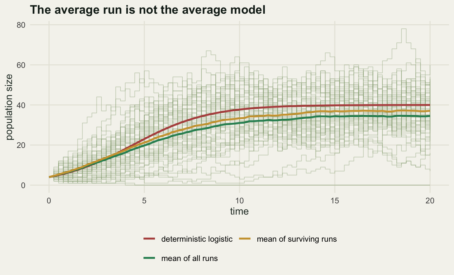
The picture makes the decomposition visible. The sage band is wide, and a few of the paths in it never left the floor. The gold curve, which averages only the survivors, sits closer to the clay deterministic curve than the green one does, and the distance still left between gold and clay at the right hand edge is the curvature term on its own. Neither summary is the deterministic solution, and neither is a typical run: at time 20 the surviving runs have a standard deviation of 8.8507 animals around a mean of 37.0839, so quoting either mean as if it were the population trajectory throws away the spread that a manager would actually act on.
Final size, which the deterministic model cannot give you
The last model is the standard stochastic SIR with a fixed host population. Susceptibles become infected at rate \(\beta S I / N\) and infected hosts recover at rate \(\gamma I\); two event types, and the same engine. With \(R_0 = \beta / \gamma\) above one the deterministic model always produces an outbreak of a size given by the final size equation \(1 - z = e^{-R_0 z}\), and always the same one. The stochastic model does something the deterministic model has no way to represent: sometimes the index case recovers before infecting anyone and nothing happens at all.
Early in an outbreak, when \(S\) is close to \(N\), each infected host is the root of an approximate branching process that produces offspring at rate \(\beta\) and stops at rate \(\gamma\), giving a mean offspring number of \(R_0\). The extinction probability of that branching process from one root is \(1/R_0\), and from \(i_0\) independent roots it is \(R_0^{-i_0}\). That prediction is available to test.
n_host <- 100; r0 <- 2; gam <- 1; bet <- r0 * gam; n_run_s <- 2000
nu_sir <- matrix(c(-1, 1, 0, -1), nrow = 2, byrow = TRUE)
rates_sir <- function(x) c(bet * x[1] * x[2] / n_host, gam * x[2])

final_size <- function(i0, n_run) {
  out <- matrix(0, n_run, 2)
  for (i in seq_len(n_run)) {
    r <- gillespie(c(n_host - i0, i0), nu_sir, rates_sir, Inf, cap = 260L)
    out[i, ] <- c((n_host - i0) - r$x[nrow(r$x), 1], r$events)
  }
  colnames(out) <- c("size", "events")
  out
}

set.seed(60219384)
sir1 <- final_size(1, n_run_s)
sir2 <- final_size(2, n_run_s)

thr <- 10
fz1 <- mean(sir1[, "size"] < thr); fz2 <- mean(sir2[, "size"] < thr)

# deterministic final size: s_inf solves s = s0 * exp(-R0 * (1 - s))
s_start <- (n_host - 1) / n_host
s_inf <- uniroot(function(s) s - s_start * exp(-r0 * (1 - s)), c(1e-6, 0.98))$root
det_size <- n_host * (s_start - s_inf)
big1 <- sir1[sir1[, "size"] >= thr, "size"]

print(round(c(hosts = n_host, R0 = r0, recovery_rate = gam,
              runs_each = n_run_s, fizzle_threshold = thr,
              fizzle_i0_1 = fz1, predicted_i0_1 = 1 / r0,
              se_i0_1 = sqrt(fz1 * (1 - fz1) / n_run_s),
              fizzle_i0_2 = fz2, predicted_i0_2 = 1 / r0^2,
              se_i0_2 = sqrt(fz2 * (1 - fz2) / n_run_s)), 4))
hosts R0 recovery_rate runs_each
100.0000 2.0000 1.0000 2000.0000
fizzle_threshold fizzle_i0_1 predicted_i0_1 se_i0_1
10.0000 0.5020 0.5000 0.0112
fizzle_i0_2 predicted_i0_2 se_i0_2
0.2505 0.2500 0.0097 gap_top <- 30
print(round(c(gap_upper_edge = gap_top,
runs_in_the_gap = sum(sir1[, "size"] >= thr & sir1[, "size"] <= gap_top),
mean_size_given_takeoff = mean(big1),
se_size_given_takeoff = sd(big1) / sqrt(length(big1)),
deterministic_final_size = det_size,
deterministic_fraction = s_start - s_inf,
shortfall_of_takeoff_runs = det_size - mean(big1),
mean_events_i0_1 = mean(sir1[, "events"]),
mean_events_i0_2 = mean(sir2[, "events"])), 4)) gap_upper_edge runs_in_the_gap mean_size_given_takeoff
30.0000 40.0000 74.6878
se_size_given_takeoff deterministic_final_size deterministic_fraction
0.4969 79.0231 0.7902
shortfall_of_takeoff_runs mean_events_i0_1 mean_events_i0_2
4.3354 76.3280 113.7740 With one index case in a population of 100 and \(R_0 = 2\), the fraction of runs that fizzled out below 10 cases is 0.502, standard error 0.0112, against the branching process prediction 0.5. With two index cases it is 0.2505, standard error 0.0097, against 0.25. The exponent is doing exactly what the theory says: two independent introductions both have to fail, and squaring a half gives a quarter.
That agreement is better than it has any right to be, and the reason deserves stating rather than celebrating. The branching approximation ignores the depletion of susceptibles, which makes take-off slightly harder than the approximation says, so the true fizzle probability should be a little above \(1/R_0\). At 100 hosts and 2000 runs that bias is smaller than the standard error of 0.0112, so this experiment cannot see it. The right reading is that the prediction survives at this precision, not that the correction is zero.
The threshold of 10 cases is not a delicate choice, because there is almost nothing to cut through. Only 40 of the 2000 runs finished with a final size between 10 and 30 cases. The distribution has a spike at the bottom and a broad hump near the top and hardly anything in between, so any threshold in that empty region gives the same answer.
The runs that did take off infected 74.6878 hosts on average, with a standard error of 0.4969. The deterministic final size equation, solved for the same starting condition, gives 79.0231 hosts. Conditioning on take-off therefore does not recover the deterministic answer either: it falls short by 4.3354 hosts, many standard errors below. Some of that gap is the company the average keeps: the 40 runs that finished between 10 and 30 cases still count as take-offs, and few as they are they sit far enough below the hump to pull the average down. Drop them and the average lifts to 77.0858 hosts, which closes about half the gap. The rest is an outbreak that survives its first few generations and still loses cases to chance on the way up, arriving at the peak with a slightly smaller infected pool than the mean field equation assumes.
fs_df <- rbind(
  data.frame(size = sir1[, "size"], panel = "one index case"),
  data.frame(size = sir2[, "size"], panel = "two index cases"))
lab_df <- data.frame(
  panel = c("one index case", "two index cases"),
  txt = c(sprintf("fizzle %.4f (predicted %.4f)", fz1, 1 / r0),
          sprintf("fizzle %.4f (predicted %.4f)", fz2, 1 / r0^2)))

ggplot(fs_df, aes(size)) +
  geom_histogram(binwidth = 4, fill = te_pal$green, colour = te_pal$paper,
                 linewidth = 0.2) +
  geom_vline(xintercept = thr, colour = te_pal$clay, linetype = 2,
             linewidth = 0.7) +
  geom_text(data = lab_df, aes(x = 50, y = Inf, label = txt),
            vjust = 1.6, colour = te_pal$ink, size = 3.4) +
  facet_wrap(~ panel) +
  labs(title = "Two outcomes, not one",
       x = "final size (hosts infected)", y = "number of runs") +
  theme_te()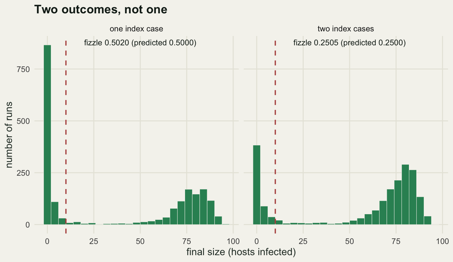
The deterministic SIR has no way to produce this picture. It gives one number, the right hand hump, and it gives it with certainty. Half of the realisations here never got there. For a manager deciding whether to act on a single detected case, the useful output is not the size of the outbreak that would follow but the probability that there will be an outbreak at all, and that probability is a property of the stochastic model only.
What exactness costs
The algorithm is exact because it visits every event. That is also the whole of its cost. The number of iterations is the number of events, and the number of events does not care how long the simulated interval is in isolation: it is the total rate integrated over that interval. Double the population and you double the rate of births and the rate of deaths, so you double the work for the same simulated time.
Never measure this with a clock. A timing number depends on the machine, the other things the machine is doing, and the phase of the moon, and it will be wrong the first time somebody else runs the code. The event count is a property of the model and the seed, and it is reproducible.
set.seed(11235813)
k_grid <- c(10, 20, 40, 80, 160)
n_rep_c <- 40
t_cost <- 10
cost_tab <- data.frame(
  K = k_grid,
  mean_events = sapply(k_grid, function(kk) {
    rl <- function(x) c(b_r * x[1], d_r * x[1] + (b_r - d_r) * x[1]^2 / kk)
    mean(replicate(n_rep_c,
      gillespie(c(kk), nu_log, rl, t_cost, cap = 20000L)$events))
  }))
cost_tab$events_per_K <- round(cost_tab$mean_events / cost_tab$K, 2)
cost_tab$mean_events <- round(cost_tab$mean_events, 1)
print(cost_tab)
K mean_events events_per_K
1 10 179.6 17.96
2 20 365.0 18.25
3 40 756.2 18.91
4 80 1566.8 19.59
5 160 3213.5 20.08print(round(c(replicates_per_K = n_rep_c, simulated_time = t_cost,
ratio_160_to_10 = cost_tab$mean_events[5] / cost_tab$mean_events[1],
ratio_of_K = k_grid[5] / k_grid[1],
large_K_limit = (b_r + d_r + (b_r - d_r)) * t_cost), 4))replicates_per_K simulated_time ratio_160_to_10 ratio_of_K
40.0000 10.0000 17.8925 16.0000
large_K_limit
20.0000 10 time units of simulation starting at carrying capacity cost 179.6 events on average when \(K\) is 10, and 3213.5 events when \(K\) is 160. The ratio of work is 17.8925 for a population ratio of 16, and the events per unit of \(K\) rise from 17.96 to 20.08 across the range. Both facts say the same thing. The cost is proportional to the population size, with a mild correction at small \(K\): at \(K\) = 10 a population sits proportionally further below its capacity than at \(K\) = 160, so it generates fewer events per animal. The large population limit is \((b + d + r)K\) per unit time, which is 20 events per unit of \(K\) over 10 time units, and the measured 20.08 has reached it to within the Monte Carlo error of 40 replicates, which is a couple of tenths of an event per unit of \(K\). The approach is from below, because a finite population spends its time a little under capacity; the last decimal of that final row is noise, not a crossing.
The rest of the post makes the same point without being asked. An immigration and death run to time 16, hovering around four animals, averaged 59.6663 events. A logistic run to time 20 with a capacity of 40 averaged 1021.432, roughly seventeen times the work for a population an order of magnitude larger held for a little longer. The epidemic runs are the interesting case: with one index case they averaged 76.328 events and with two index cases 113.774, and the difference is not that two infectives spread faster but that half as many runs die out in the first few events. Cheap runs are cheap because nothing happens in them, which is also why the total cost of a stochastic study is hard to guess in advance.
That is the practical limit of the method. A model of a few hundred individuals is comfortable. A model of a hundred thousand, run for a season, is not: you would be asking base R for tens of millions of loop iterations to get one trajectory. This is precisely the situation where tau leaping earns its keep, holding the propensities fixed over a short window and drawing a Poisson number of firings of each event type instead of stepping through them one at a time. That is an approximation, it has an error you can measure, and it is the subject of the next post. The point of building the exact algorithm first is that you now have something to measure the approximation against.
What to take away
The exact algorithm is short enough to write from memory: total rate, exponential waiting time, categorical choice of event, update, repeat. The value of writing it yourself is that every assumption is visible in the rates function, and there is no step size hiding an error term. When it matters that populations are integers, and it matters most near zero, this is the sampler that gets the answer right rather than nearly right.
The measurements here also make a case for how to check any sampler. Almost every comparison in this post is against a closed form rather than against another simulation: the maximum of ten exponentials for the pure death process, the Poisson law for immigration and death, where the simulated distribution sat 0.017 in total variation from the exact law while perfect samples of the same size sit at 0.0216 on average, the branching process fizzle probability for the epidemic, and the moment identity for the logistic. Only one comparison, direct method against first reaction, put two samplers side by side, and that is the weakest of the set as well as the one most people actually run.
The honest limit is the one that no amount of exactness fixes. The algorithm samples exactly from the model it is given, and the model is a claim that between events the rate of every event type is a fixed function of the current counts; nothing in this post tests that claim against a real population, where rates vary with weather, age, spatial arrangement and the memory of what happened last month. The stochastic logistic reproduced its own moment identity to within 0.7383 animals, with the shortfall pointing the way it should when the mean has not quite settled. That says the code does what the model says. It says nothing at all about whether a pond of newts obeys the model. Exact simulation of a wrong model is still a wrong answer, delivered one event at a time.
References
Gillespie DT 1976 Journal of Computational Physics 22(4):403-434 (10.1016/0021-9991(76)90041-3)
Gillespie DT 1977 The Journal of Physical Chemistry 81(25):2340-2361 (10.1021/j100540a008)
Gillespie DT 2001 The Journal of Chemical Physics 115(4):1716-1733 (10.1063/1.1378322)
Anderson RM, May RM 1991 Infectious Diseases of Humans: Dynamics and Control (ISBN 978-0-19-854040-3)
Nasell I 2001 Journal of Theoretical Biology 211(1):11-27 (10.1006/jtbi.2001.2328)
Keeling MJ, Rohani P 2008 Modeling Infectious Diseases in Humans and Animals (ISBN 978-0-691-11617-4)
Black AJ, McKane AJ 2012 Trends in Ecology and Evolution 27(6):337-345 (10.1016/j.tree.2012.01.014)