library(ggplot2)

te_pal <- list(forest = "#275139", green = "#2f8f63", sage = "#93a87f",
               clay = "#b5534e", gold = "#cda23f", line = "#dad9ca",
               ink = "#16241d", paper = "#f5f4ee")

theme_te <- function() {
  theme_minimal(base_size = 12) +
    theme(panel.grid.minor = element_blank(),
          panel.grid.major = element_line(colour = "#e7e6dc"),
          plot.background = element_rect(fill = "#f5f4ee", colour = NA),
          panel.background = element_rect(fill = "#f5f4ee", colour = NA),
          plot.title = element_text(face = "bold", colour = te_pal$ink),
          axis.title = element_text(colour = "#2c3a31"),
          legend.position = "bottom")
}Tau leaping and the cost of a bigger step
R
stochastic simulation
population models
ecology tutorial
Tau leaping in base R: measuring what a larger simulation step costs in the mean, the variance and the whole distribution of an ecological birth-death model.
There are eight concrete cattle troughs along a farm track near the field station, filled by rain and by an intermittent pipe, and each spring they are colonised by diving beetles that fly in from a permanent pond about four hundred metres away. Somebody counts them every fortnight. The counts sit around twenty per trough and wobble by five or six between visits, which is exactly what you expect from a patch that gains individuals at a roughly constant rate from outside and loses them at a rate proportional to how many are already there.
That is the simplest island model there is, and it has a property that makes it extremely useful for testing simulation code: you know the answer. Constant immigration plus a constant per capita death rate gives a stationary distribution that is Poisson with mean equal to the immigration rate over the death rate. Not approximately Poisson. Exactly Poisson, for every parameter value. So any simulator you write can be marked against a distribution you can type out in one line.
The reason to care is that the exact simulation algorithm, which draws one event at a time and advances the clock by an exponential waiting time, does an amount of work proportional to the total event rate. For eight troughs of twenty beetles that is nothing. For a population of ten million, or for a metapopulation of two thousand patches, the exact algorithm simulates every single birth and death and becomes unaffordable long before the biology gets interesting. Tau leaping is the standard escape: fix a step of length tau, and over that step draw the number of events of each type from a Poisson distribution whose mean is the propensity times tau, computed from the state at the start of the step. Beyond that lies the ordinary differential equation, which takes the limit and drops the noise entirely.
This post measures what those two approximations cost. Not in seconds, because seconds depend on the machine and on what else it is doing, but in the currency that transfers: the number of random draws needed, set against the error in the answer. The result that came out of the measurement and that I did not expect is that the two things that go wrong with a big step go wrong in opposite directions with population size. The crash that everybody warns about is a small-population problem. The error that actually corrupts your inference gets worse as the population grows.
The exact sampler is built and validated in The Gillespie algorithm from scratch; here it is written out again compactly so this post stands alone.
Two samplers for the same trough
The model has one state variable, the number of beetles n in a trough, and two event types. Immigration happens at rate imm, independent of n. Death happens at rate mort * n. I will use an immigration rate of twenty per unit time and a per capita death rate of one, so the equilibrium is twenty beetles and the natural timescale of the process is one time unit.
imm  <- 20
mort <- 1
n_eq <- imm / mort
print(round(c(immigration_rate = imm, death_rate_per_capita = mort,
              equilibrium = n_eq, exact_variance = n_eq), 4))
immigration_rate death_rate_per_capita equilibrium
20 1 20
exact_variance
20 The exact algorithm is the direct method. Total propensity, exponential waiting time, then a uniform draw to decide which of the two events fired. The leap is the same model seen through a wider aperture: hold the propensities fixed at their start-of-step values, and draw the number of immigrations and the number of deaths over the whole step from independent Poisson distributions.
ssa_run <- function(n0, t_end) {
  times <- counts <- numeric(60000L)
  k <- 1L; times[1] <- 0; counts[1] <- n0; tnow <- 0; n <- n0; nev <- 0L
  while (TRUE) {
    a0 <- imm + mort * n
    tnow <- tnow + rexp(1, a0)
    if (tnow > t_end) break
    if (runif(1) * a0 < imm) n <- n + 1 else n <- n - 1
    nev <- nev + 1L
    k <- k + 1L
    times[k] <- tnow; counts[k] <- n
  }
  list(times = times[1:k], n = counts[1:k], events = nev)
}

leap_run <- function(n0, tau, t_end, guard = TRUE) {
  nstep <- floor(t_end / tau)
  out <- numeric(nstep + 1L); out[1] <- n0
  n <- n0; draws <- 0L
  for (s in seq_len(nstep)) {
    n_imm <- rpois(1, imm * tau)
    n_die <- rpois(1, mort * n * tau)
    draws <- draws + 2L
    if (guard) n_die <- min(n_die, n)
    n <- n + n_imm - n_die
    out[s + 1L] <- n
  }
  list(times = (0:nstep) * tau, n = out, draws = draws)
}

set.seed(20260728)
one_exact <- ssa_run(2, 15)
one_leap  <- leap_run(2, 0.5, 15)
print(round(c(exact_events = one_exact$events,
              leap_draws = one_leap$draws,
              leap_steps = length(one_leap$n) - 1), 4))
exact_events leap_draws leap_steps
585 60 30 Fifteen time units of the exact process took 585 individual events. The leap with a step of 0.5 covered the same fifteen time units in 30 steps and 60 Poisson draws. That ratio is the whole promise of the method, and the rest of this post is about what it costs.
The deterministic version needs no simulation at all. With immigration imm and per capita mortality mort, the mean field equation is dn/dt = imm - mort * n, whose solution from a starting count n0 is n_eq + (n0 - n_eq) * exp(-mort * t).
ode_t <- seq(0, 15, length.out = 400)
lab <- c("exact algorithm", "tau leap, step 0.5", "deterministic")
traj <- data.frame(
  time  = c(one_exact$times, one_leap$times, ode_t),
  count = c(one_exact$n, one_leap$n, n_eq + (2 - n_eq) * exp(-mort * ode_t)),
  series = factor(rep(lab, c(length(one_exact$times), length(one_leap$times),
                             length(ode_t))), levels = lab))

ggplot(traj, aes(time, count, colour = series)) +
  geom_step(data = subset(traj, series != "deterministic"), linewidth = 0.5) +
  geom_line(data = subset(traj, series == "deterministic"), linewidth = 1.1) +
  scale_colour_manual(values = c(te_pal$forest, te_pal$clay, te_pal$gold),
                      name = NULL) +
  labs(title = "Same model, three levels of detail",
       x = "time", y = "beetles in the trough") +
  theme_te()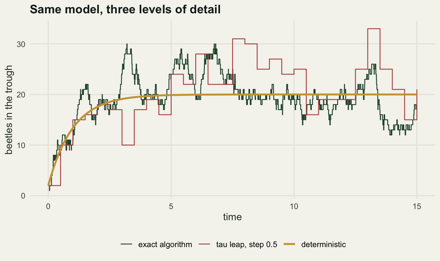
The leaped path in the figure is visibly coarser: it only changes value at multiples of 0.5, and when it changes it can move several individuals at once. What is much harder to see by eye is whether its long run behaviour is right. The path looks plausible. Plausible is not a measurement.
The step that takes the count below zero
Before any accuracy question there is a correctness question that a surprising amount of published leap code gets wrong. The number of deaths over the step is drawn from a Poisson distribution with mean mort * n * tau. A Poisson variable has no upper bound. Nothing stops it from returning more deaths than there are individuals, and when it does, the state goes negative, the next death propensity is negative, and rpois is asked for a negative mean.
How often does that actually happen? I ran the unguarded leap from equilibrium for sixty time units, four hundred independent chains per cell, and recorded the fraction of chains that produced a negative count at least once, plus the per step rate.
set.seed(20260728)
crash_scan <- function(kk, tau, t_end, nrep) {
  n <- rep(kk, nrep); alive <- rep(TRUE, nrep)
  nstep <- floor(t_end / tau); steps_done <- 0
  for (s in seq_len(nstep)) {
    k <- which(alive)
    if (!length(k)) break
    steps_done <- steps_done + length(k)
    prop <- n[k] + rpois(length(k), kk * tau) - rpois(length(k), n[k] * tau)
    bad <- prop < 0
    alive[k[bad]] <- FALSE
    n[k[!bad]] <- prop[!bad]
  }
  c(equilibrium = kk, tau = tau, chains_crashed = mean(!alive),
    per_step_rate = sum(!alive) / steps_done)
}

n_chains <- 400
horizon  <- 60
cells <- expand.grid(tau = c(0.1, 0.25, 0.5, 1), equilibrium = c(5, 20, 80))
crash <- as.data.frame(t(mapply(function(kk, tt)
  crash_scan(kk, tt, horizon, n_chains), cells$equilibrium, cells$tau)))
print(round(crash, 6))
equilibrium tau chains_crashed per_step_rate
1 5 0.10 0.1150 0.000203
2 5 0.25 0.2475 0.001171
3 5 0.50 0.6050 0.007805
4 5 1.00 0.9375 0.044484
5 20 0.10 0.0000 0.000000
6 20 0.25 0.0000 0.000000
7 20 0.50 0.0000 0.000000
8 20 1.00 0.0400 0.000681
9 80 0.10 0.0000 0.000000
10 80 0.25 0.0000 0.000000
11 80 0.50 0.0000 0.000000
12 80 1.00 0.0000 0.000000pick_crash <- function(kk, tt)
100 * crash$chains_crashed[crash$equilibrium == kk & crash$tau == tt]
crash_pct <- c(eq5_step_half = pick_crash(5, 0.5), eq5_step_one = pick_crash(5, 1),
eq20_step_one = pick_crash(20, 1), eq80_step_one = pick_crash(80, 1))
print(round(crash_pct, 2))eq5_step_half eq5_step_one eq20_step_one eq80_step_one
60.50 93.75 4.00 0.00 print(round(c(chains_per_cell = n_chains, time_horizon = horizon), 4))chains_per_cell time_horizon
400 60 Read the chains_crashed column down the equilibrium blocks. At an equilibrium of five beetles the unguarded leap is a disaster: with a step of 0.5, 60.5 per cent of the four hundred chains hit a negative count within sixty time units, and with a step of 1 it is 93.75 per cent. At an equilibrium of twenty only the step of 1 produces any crashes at all, and only in 4 per cent of chains. At an equilibrium of eighty, not one chain out of four hundred went negative at any of the four steps tested.
That is the opposite of the impression the literature gives. The negative-count failure is loud and easy to detect, which is why it gets the attention, but it is a small-population phenomenon. A crash needs the death draw to exceed the immigration draw by more than the current count, and the gap between those two draws has a standard deviation of about the square root of twice the equilibrium times tau while the count itself is of order the equilibrium. Larger populations push the crash out into the tail, fast. If your model has thousands of individuals you will never see this failure, and you may conclude your step size is fine.
Two repairs are standard. The first caps each event count at the number of individuals available, so the death count becomes min(n_die, n). The second shrinks tau until the crashes stop. Both are easy to code. They are not equivalent, and the difference is not in the crash rate but in the answer.
What a bigger step costs the answer
To measure the answer rather than a sample of it, note that the guarded fixed-step leap is itself a Markov chain on the non-negative integers, with a transition kernel you can write down: from state n the new state is n minus a capped Poisson death count plus a Poisson immigration count, which is a convolution of two known distributions. Build the transition matrix, solve for the stationary distribution, and you have the leap’s exact long run law with no Monte Carlo error at all. Then compare it to the Poisson that the exact process gives.
leap_matrix <- function(up, dn, tau, nmax) {
  ns <- nmax + 1L
  kern <- matrix(0, ns, ns)
  for (k in seq_len(ns)) {
    n <- k - 1L
    lam_up <- up(n) * tau; lam_dn <- dn(n) * tau
    imax <- qpois(1 - 1e-13, max(lam_up, 1e-12)) + 6L
    p_up <- dpois(0:imax, lam_up)
    p_up[imax + 1L] <- p_up[imax + 1L] + (1 - sum(p_up))
    p_surv <- 1
    if (n > 0L) {
      p_dn <- dpois(0:n, lam_dn)
      p_dn[n + 1L] <- p_dn[n + 1L] + (1 - sum(p_dn))   # the cap
      p_surv <- rev(p_dn)
    }
    cv <- convolve(p_surv, rev(p_up), type = "open")
    cv[cv < 0] <- 0
    idx <- seq_along(cv) - 1L
    idx[idx > nmax] <- nmax
    agg <- rowsum(cv, idx); row <- numeric(ns)
    row[as.integer(rownames(agg)) + 1L] <- agg[, 1]
    kern[k, ] <- row / sum(row)
  }
  kern
}

stat_dist <- function(kern) {
  ns <- nrow(kern)
  amat <- t(kern) - diag(ns)
  amat[ns, ] <- 1
  ps <- solve(amat, c(numeric(ns - 1L), 1))
  ps[ps < 0] <- 0
  ps / sum(ps)
}

moments_of <- function(ps) {
  x <- seq_along(ps) - 1
  m <- sum(ps * x)
  c(mean = m, variance = sum(ps * (x - m)^2))
}

tv_dist <- function(p, q) 0.5 * sum(abs(p - q))
Before trusting the algebra, check it against the thing it claims to describe. I ran four hundred guarded leap chains at a step of 0.25, discarded a burn-in of twenty time units, and sampled the state every four time units afterwards.
set.seed(20260729)
mc_leap <- function(tau, t_end, burn, thin, nrep) {
  n <- rep(n_eq, nrep); nstep <- floor(t_end / tau); keep <- numeric(0)
  for (s in seq_len(nstep)) {
    n_die <- pmin(rpois(nrep, mort * n * tau), n)
    n <- n + rpois(nrep, imm * tau) - n_die
    tt <- s * tau
    if (tt > burn && abs(tt / thin - round(tt / thin)) < 1e-9) keep <- c(keep, n)
  }
  keep
}
samp <- mc_leap(0.25, 220, 20, 4, 400)
kern_check <- leap_matrix(function(n) imm, function(n) mort * n, 0.25, 200)
mom_check  <- moments_of(stat_dist(kern_check))
print(round(c(step_checked = 0.25, mc_mean = mean(samp),
              kernel_mean = mom_check[["mean"]],
              mc_variance = var(samp), kernel_variance = mom_check[["variance"]],
              n_samples = length(samp)), 4))
step_checked mc_mean kernel_mean mc_variance kernel_variance
0.2500 20.0108 20.0000 23.2721 22.8567
n_samples
20000.0000 The 20000 simulated states give a mean of 20.0108 against the kernel’s 20, and a variance of 23.2721 against the kernel’s 22.8567. The kernel is describing the same chain the simulation runs, so from here on I use the kernel and stop paying Monte Carlo noise.
Now the sweep: ten step sizes spanning a little over two orders of magnitude, and three error measures. The relative error in the mean, the relative error in the variance (both expressed relative to the true value of twenty), and the total variation distance between the leap’s stationary distribution and the exact Poisson.
nmax1 <- 200
exact1 <- dpois(0:nmax1, n_eq); exact1 <- exact1 / sum(exact1)
taus <- 10^seq(log10(0.005), log10(1), length.out = 10)

sweep_one <- function(tau) {
  ps <- stat_dist(leap_matrix(function(n) imm, function(n) mort * n, tau, nmax1))
  mo <- moments_of(ps)
  nn <- 0:nmax1
  c(tau = tau,
    mean_err = abs(mo[["mean"]] - n_eq) / n_eq,
    var_err  = abs(mo[["variance"]] - n_eq) / n_eq,
    tv       = tv_dist(ps, exact1),
    cap_rate = sum(ps * ppois(nn, mort * nn * tau, lower.tail = FALSE)))
}
tau_sweep <- as.data.frame(t(sapply(taus, sweep_one)))
tau_sweep$bias_per_guard <- (tau_sweep$mean_err * n_eq) /
                            (tau_sweep$cap_rate / tau_sweep$tau)
print(signif(tau_sweep, 4))
tau mean_err var_err tv cap_rate bias_per_guard
1 0.005000 6.292e-12 0.002506 0.0006125 6.356e-13 0.9898
2 0.009008 1.355e-11 0.004524 0.0011050 2.437e-12 1.0020
3 0.016230 3.297e-11 0.008181 0.0019930 1.064e-11 1.0060
4 0.029240 1.008e-10 0.014840 0.0036020 5.818e-11 1.0130
5 0.052680 4.553e-10 0.027050 0.0065260 4.667e-10 1.0280
6 0.094910 3.901e-09 0.049820 0.0118800 6.980e-09 1.0610
7 0.171000 8.791e-08 0.093490 0.0217900 2.644e-07 1.1370
8 0.308100 6.677e-06 0.182000 0.0405600 3.122e-05 1.3180
9 0.555000 1.197e-03 0.368100 0.0773000 7.289e-03 1.8220
10 1.000000 9.220e-02 0.345200 0.1471000 4.422e-01 4.1700head_pct <- c(var_pct_mid = 100 * tau_sweep$var_err[5],
var_pct_at_step7 = 100 * tau_sweep$var_err[7],
var_pct_at_step8 = 100 * tau_sweep$var_err[8],
guard_pct_at_step10 = 100 * tau_sweep$cap_rate[10],
mean_pct_at_step10 = 100 * tau_sweep$mean_err[10],
var_over_mean_at_step7 = tau_sweep$var_err[7] / tau_sweep$mean_err[7])
print(signif(head_pct, 4)) var_pct_mid var_pct_at_step7 var_pct_at_step8
2.705e+00 9.349e+00 1.820e+01
guard_pct_at_step10 mean_pct_at_step10 var_over_mean_at_step7
4.422e+01 9.220e+00 1.064e+06 print(round(c(n_steps_swept = length(taus), state_space_top = nmax1), 4)) n_steps_swept state_space_top
10 200 The steps run from 0.005 to 1. The variance column is the one to look at first. At a step of 0.0527 the leap’s stationary variance is already 2.705 per cent too large; at 0.3081 it is 18.2 per cent too large. The leap does not add noise in a vague sense: it inflates the variance in a specific and predictable way, because holding the death propensity fixed for the whole step removes the within-step negative feedback that pulls a high count back down.
The mean column is the surprise. At a step of 0.171, where the variance is already 9.349 per cent wrong, the relative error in the mean is \(8.79 \times 10^{-8}\). The variance error at that step is about \(1.06 \times 10^{6}\) times larger than the mean error. That is not a tuning difference. That is a different regime.
The reason is worth being precise about, because it is the whole content of the section. The expected change over a step, immigration times tau minus death rate times count times tau, is linear in the count, so it commutes with taking expectations: the leap’s drift is the true drift, exactly, at every step size. An unguarded leap on this model would reproduce the mean of 20 to machine precision for any tau you like. Every bit of the mean error in the table is put there by the guard.
The last two columns show that directly. cap_rate is the stationary probability that the death draw exceeds the available count, that is, the probability per step that the guard fires; it stays below one in a million until the step reaches 0.3081. bias_per_guard divides the absolute bias in the mean by the guard’s firing rate per unit time, and over the small-step half of the sweep it sits at 0.9898 to 1.028. In words: each time the guard fires it hands back about one individual that the Poisson draw wanted to kill twice, and that individual then sits in the population for about one relaxation time before it leaves. By a step of 1 the guard fires on 44.22 per cent of steps, the ratio has risen to 4.17 because the guard now fires repeatedly before the population recovers, and the mean is 9.22 per cent too high.
So the bias in the mean is not the leap’s error at any step. It is the repair’s error, and it is governed by a Poisson tail probability rather than by tau itself. That also settles the choice between the two repairs. Capping keeps the cheap step and pays for it with a biased mean; shrinking tau keeps the mean and pays in draws.
err_at <- function(kk, tau) {
  nmax <- ceiling(kk + 12 * sqrt(kk / max(0.05, 1 - tau / 2)) + 25)
  ex <- dpois(0:nmax, kk); ex <- ex / sum(ex)
  ps <- stat_dist(leap_matrix(function(n) kk, function(n) n, tau, nmax))
  mo <- moments_of(ps)
  nn <- 0:nmax
  c(tau = tau, mean_err = (mo[["mean"]] - kk) / kk,
    var_err = (mo[["variance"]] - kk) / kk, tv = tv_dist(ps, ex),
    cap_rate = sum(ps * ppois(nn, nn * tau, lower.tail = FALSE)),
    boundary_mass = ps[nmax + 1L])
}
shrink <- c(0.5, 0.25, 0.125, 0.0625)
rep_tab <- as.data.frame(t(sapply(shrink, function(x) err_at(5, x))))
print(signif(rep_tab, 4))
tau mean_err var_err tv cap_rate boundary_mass
1 0.5000 0.0252200 0.23290 0.054020 4.482e-02 0
2 0.2500 0.0040900 0.12460 0.030510 4.461e-03 0
3 0.1250 0.0009863 0.06200 0.015540 5.825e-04 0
4 0.0625 0.0003273 0.03067 0.007773 9.976e-05 0repair_pct <- c(big_step_mean = 100 * rep_tab$mean_err[1],
big_step_var = 100 * rep_tab$var_err[1],
small_step_mean = 100 * rep_tab$mean_err[4],
small_step_var = 100 * rep_tab$var_err[4])
print(signif(repair_pct, 4)) big_step_mean big_step_var small_step_mean small_step_var
2.52200 23.29000 0.03273 3.06700 set.seed(20260730)
rep_crash <- as.data.frame(t(sapply(shrink, function(x)
crash_scan(5, x, horizon, n_chains))))
print(round(rep_crash, 6)) equilibrium tau chains_crashed per_step_rate
1 5 0.5000 0.5525 0.006781
2 5 0.2500 0.3250 0.001642
3 5 0.1250 0.1725 0.000394
4 5 0.0625 0.0775 0.000084print(round(c(crashed_pct_big_step = 100 * rep_crash$chains_crashed[1],
crashed_pct_small_step = 100 * rep_crash$chains_crashed[4]), 2)) crashed_pct_big_step crashed_pct_small_step
55.25 7.75 At an equilibrium of five, the population size where the crash was worst, the capped leap with a step of 0.5 gets a mean that is 2.522 per cent too high, a variance 23.29 per cent too high, and a total variation distance of 0.05402 from the truth. Shrinking the step by a factor of eight to 0.0625 brings the mean bias down to 0.03273 per cent and the variance error to 3.067 per cent, at eight times the number of draws.
The crash table underneath is an independent set of 400 chains, so it differs from the grid above by Monte Carlo noise alone: the same cell, an equilibrium of five with a step of 0.5, comes out at 55.25 per cent here against 60.5 per cent there. Shrinking the step by a factor of eight reduces the fraction of unguarded chains that die from 55.25 per cent to 7.75 per cent. It does not reach zero, because the chain still wanders down to two or three beetles now and then, and at two or three beetles almost any step is a large step. Shrinking tau globally is an expensive fix for a problem that lives only in the lower tail. The cap is the better repair; you just have to know that it moves the mean, and check how often it fires.
The order of convergence, fitted rather than assumed
Textbook accounts say the fixed-step leap is first order. Better to check that against the numbers than to take it, so I regressed log error on log tau over the part of the sweep where the guard is effectively never firing.
clean <- which(tau_sweep$cap_rate < 1e-5)
fit_slope <- function(y, keep)
  unname(coef(lm(log(y[keep]) ~ log(tau_sweep$tau[keep])))[2])
three <- function(keep) c(mean = fit_slope(tau_sweep$mean_err, keep),
                          variance = fit_slope(tau_sweep$var_err, keep),
                          total_variation = fit_slope(tau_sweep$tv, keep))
slopes <- three(clean)
print(round(slopes, 4))
mean variance total_variation
2.5835 1.0223 1.0101 local_slopes <- rbind(smaller_half = three(clean[1:4]),
larger_half = three(clean[(length(clean) - 3):length(clean)]))
print(round(local_slopes, 4)) mean variance total_variation
smaller_half 1.5646 1.0068 1.0032
larger_half 3.8154 1.0418 1.0188print(round(c(points_used = length(clean)), 4))points_used
7 Over the 7 step sizes where the guard fires less than once in a hundred thousand steps, the relative error in the variance scales as tau to the power 1.0223 and the total variation distance as tau to the power 1.0101. Both are first order, so the textbook is right about those two.
The mean is not a power law at all, and the second table is the evidence. Fitting the whole clean range gives an exponent of 2.5835, but that single number is a fiction: over the four smallest steps the local exponent is 1.5646 and over the four largest it is 3.8154, more than double. The variance and the total variation distance show no such drift, moving from 1.0068 to 1.0418 and from 1.0032 to 1.0188. A curve whose local slope keeps steepening is what a tail probability looks like on log axes, which is what the guard’s firing rate is. Quote a convergence order for the mean here and you are quoting a number that depends on which steps you happened to try.
The practical reading of a first order method is blunt: halving the step halves the error and doubles the work, so the accuracy you get is set by the work you are willing to do, and there is no step size at which the leap suddenly becomes accurate.
meas <- c("error in the mean", "error in the variance",
          "total variation distance")
err_long <- data.frame(
  tau = rep(tau_sweep$tau, 3),
  err = c(tau_sweep$mean_err, tau_sweep$var_err, tau_sweep$tv),
  measure = factor(rep(meas, each = nrow(tau_sweep)), levels = meas))

ggplot(err_long, aes(tau, err, colour = measure, shape = measure)) +
  geom_line(linewidth = 0.6) +
  geom_point(size = 2.4) +
  scale_x_log10() +
  scale_y_log10() +
  scale_colour_manual(values = c(te_pal$forest, te_pal$clay, te_pal$gold),
                      name = NULL) +
  scale_shape_manual(values = c(15, 16, 17), name = NULL) +
  labs(title = "The mean is free, the spread is not",
       x = "step size tau", y = "error") +
  theme_te() +
  theme(legend.box = "vertical")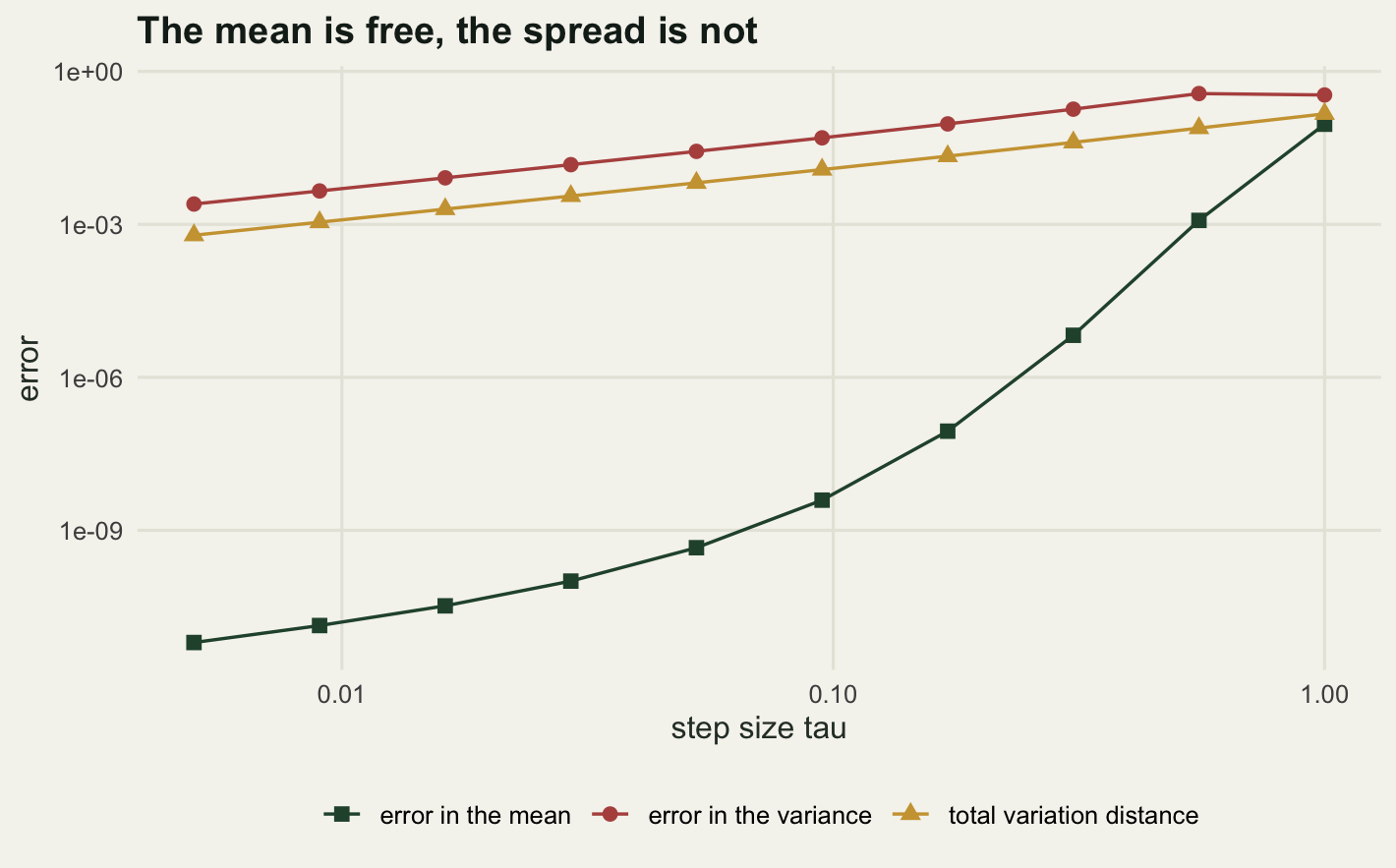
The figure makes the asymmetry impossible to miss. If you tuned your step size by simulating, looking at the mean and comparing it to what you expected, this model would tell you that a step of 1 is fine, while the variance at that step is wrong by tens of per cent.
That matters because of why people run stochastic population models at all. Nobody simulates a birth-death process to learn the equilibrium; the deterministic model gives that for free. They simulate it to get the spread: the probability of falling below a threshold, the variance of an abundance index, the quantiles of a time to extinction. Those are functions of exactly the part of the answer the leap damages first.
Cost, counted in draws rather than seconds
Timing code is not portable, so count draws instead. The exact algorithm uses two random numbers per event (one exponential for the waiting time, one uniform to pick the event), and at stationarity the total propensity is immigration plus deaths, which averages twice the immigration rate. The leap uses two Poisson draws per step regardless of the state, and takes one over tau steps per unit time.
set.seed(20260731)
ssa_events <- sapply(1:30, function(i) ssa_run(round(n_eq), horizon)$events)
print(round(c(ssa_runs = 30, mean_events_per_time = mean(ssa_events) / horizon,
              expected_total_propensity = 2 * imm), 4))
ssa_runs mean_events_per_time expected_total_propensity
30.0000 39.6761 40.0000 work_tab <- function(kk) {
tt <- c(0.01, 0.025, 0.05, 0.1, 0.25, 0.5)
out <- t(sapply(tt, function(x) err_at(kk, x)))
data.frame(equilibrium = kk, tau = tt,
draws_per_time = 2 / tt,
exact_draws_per_time = 4 * kk,
speedup = (4 * kk) / (2 / tt),
var_err = out[, "var_err"])
}
work <- rbind(work_tab(20), work_tab(320))
print(signif(work, 4)) equilibrium tau draws_per_time exact_draws_per_time speedup var_err
1 20 0.010 200 80 0.4 0.005025
2 20 0.025 80 80 1.0 0.012660
3 20 0.050 40 80 2.0 0.025640
4 20 0.100 20 80 4.0 0.052630
5 20 0.250 8 80 10.0 0.142800
6 20 0.500 4 80 20.0 0.326600
7 320 0.010 200 1280 6.4 0.005025
8 320 0.025 80 1280 16.0 0.012660
9 320 0.050 40 1280 32.0 0.025640
10 320 0.100 20 1280 64.0 0.052630
11 320 0.250 8 1280 160.0 0.142900
12 320 0.500 4 1280 320.0 0.333300pick <- function(kk, tt) work[work$equilibrium == kk & abs(work$tau - tt) < 1e-12, ]
w_break <- pick(20, 0.025)
w_ten <- pick(20, 0.25)
w_big <- pick(320, 0.025)
leap_gap <- max(abs(work$var_err[work$equilibrium == 20] -
work$var_err[work$equilibrium == 320]))
print(signif(c(exact_draws_eq20 = 2 * mean(ssa_events) / horizon,
max_gap_between_leap_curves = leap_gap,
breakeven_tau = w_break$tau,
breakeven_var_pct = 100 * w_break$var_err,
tenfold_tau = w_ten$tau, tenfold_var_pct = 100 * w_ten$var_err,
big_tau = w_big$tau, big_speedup = w_big$speedup,
big_var_pct = 100 * w_big$var_err), 5)) exact_draws_eq20 max_gap_between_leap_curves
79.3520000 0.0067347
breakeven_tau breakeven_var_pct
0.0250000 1.2658000
tenfold_tau tenfold_var_pct
0.2500000 14.2840000
big_tau big_speedup
0.0250000 16.0000000
big_var_pct
1.2658000 Thirty exact runs of sixty time units averaged 39.676 events per unit time, against the expected total propensity of 40. Each event costs two random numbers, so the exact algorithm at an equilibrium of twenty spends about 79.352 draws per unit of simulated time.
The leap breaks even against that at a step of 0.025, where it also spends 80 draws per unit time, and at that step its variance is already 1.2658 per cent wrong. To get a tenfold saving at this population size you need a step of 0.25, which costs 14.284 per cent in the variance. At an equilibrium of twenty beetles, tau leaping is a bad deal: just run the exact algorithm.
The picture changes when the population does. The exact algorithm’s cost grows in proportion to the population, because it simulates every event; the leap’s cost at fixed tau does not depend on the population at all. At an equilibrium of 320 the exact algorithm needs 1280 draws per unit time, so a step of 0.025 gives a 16-fold saving for 1.2658 per cent in the variance. That is a good trade, and it is the trade the method exists to make.
work$label <- paste("leap, equilibrium", work$equilibrium)
series_lv <- c("leap, equilibrium 20", "leap, equilibrium 320", "exact algorithm")
pts <- rbind(work[, c("draws_per_time", "var_err", "label")],
             data.frame(draws_per_time = c(80, 1280), var_err = 0,
                        label = "exact algorithm"))
pts$label <- factor(pts$label, levels = series_lv)

ggplot(pts, aes(draws_per_time, var_err,
                colour = label, shape = label, linetype = label)) +
  geom_line(data = subset(pts, label != "exact algorithm"), linewidth = 0.8) +
  geom_point(aes(size = label), stroke = 1.1) +
  annotate("text", x = c(80, 1280), y = -0.031, size = 3.2,
           label = c("eq. 20", "eq. 320"), colour = te_pal$ink) +
  scale_x_log10(expand = expansion(mult = c(0.10, 0.20))) +
  scale_y_continuous(expand = expansion(mult = c(0.18, 0.06))) +
  scale_colour_manual(values = c(te_pal$clay, te_pal$green, te_pal$ink),
                      name = NULL) +
  scale_shape_manual(values = c(16, 1, 18), name = NULL) +
  scale_linetype_manual(values = c("solid", "22", "blank"), name = NULL) +
  scale_size_manual(values = c(2.2, 4.4, 4.2), name = NULL) +
  labs(title = "Error against work, no clock involved",
       x = "random draws per unit of simulated time",
       y = "relative error in the variance") +
  theme_te()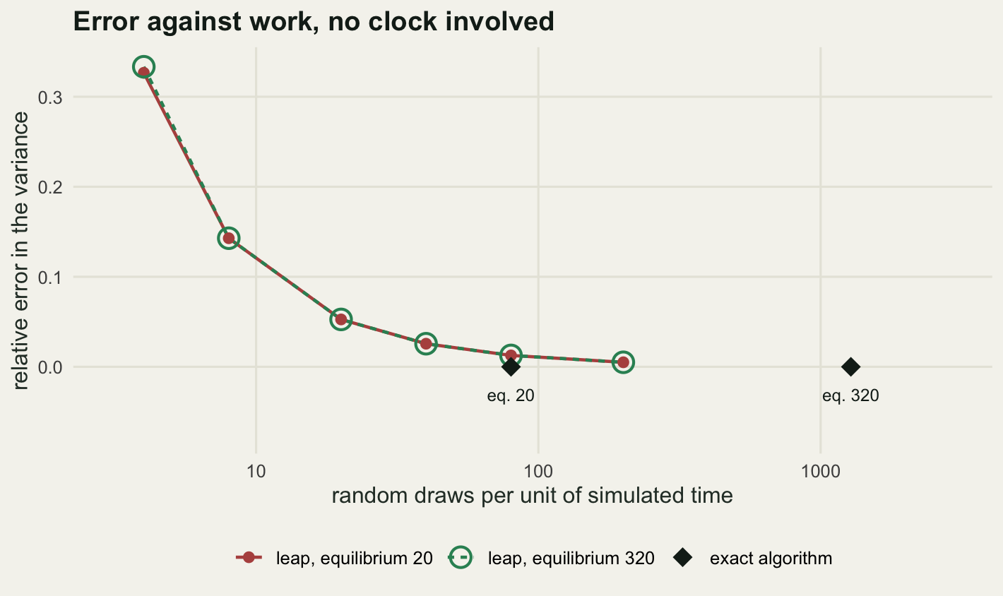
The two leap curves lie almost on top of each other, which is the point: the widest gap between them anywhere in the figure is 0.0067 in relative error, at the coarsest step, where the guard fires often enough at an equilibrium of twenty to shave the variance a little. Only the exact algorithm’s cost moves with the population. The eq. 20 diamond needs reading carefully, though, because it does not sit to the right of its curve: at 80 draws per unit time the two methods cost the same, and there the exact algorithm has no error while the leap is 1.2658 per cent wrong in the variance. The leap curve then runs on past the diamond, spending more for a worse answer. Tau leaping does not become more accurate in large populations; it becomes cheaper relative to an alternative whose price has gone up.
Does the leap condition deliver what it promises?
The standard way to choose tau is a leap condition: pick the largest step over which no propensity is expected to change by more than a small fraction of itself. The usual implementation bounds the expected change and the standard deviation of the change in each species count by max(eps * n, 1), and takes the smaller of the two resulting step limits. Here is that rule for a one-species system, evaluated over the central ninety per cent of the true stationary distribution so it reflects the states the chain actually visits.
tau_rule <- function(kk, eps) {
  nn <- qpois(0.05, kk):qpois(0.95, kk)
  drift <- kk - nn
  spread <- kk + nn
  bnd <- pmax(eps * nn, 1)
  min(pmin(ifelse(drift == 0, Inf, bnd / abs(drift)), bnd^2 / spread))
}

grid_lc <- expand.grid(eps = c(0.02, 0.05, 0.1), equilibrium = c(5, 20, 80, 320))
lc <- do.call(rbind, Map(function(kk, eps) {
  tr <- tau_rule(kk, eps)
  e <- err_at(kk, tr)
  data.frame(equilibrium = kk, eps = eps, tau_chosen = tr,
             var_err = e[["var_err"]], tv = e[["tv"]],
             boundary_mass = e[["boundary_mass"]])
}, grid_lc$equilibrium, grid_lc$eps))
print(signif(lc, 4))
equilibrium eps tau_chosen var_err tv boundary_mass
1 5 0.02 0.07143 0.035110 0.008886 0.000e+00
2 5 0.05 0.07143 0.035110 0.008886 0.000e+00
3 5 0.10 0.07143 0.035110 0.008886 0.000e+00
4 20 0.02 0.02083 0.010530 0.002562 0.000e+00
5 20 0.05 0.02500 0.012660 0.003077 1.036e-17
6 20 0.10 0.05121 0.026280 0.006342 0.000e+00
7 80 0.02 0.01193 0.006003 0.001451 0.000e+00
8 80 0.05 0.07459 0.038740 0.009212 9.075e-17
9 80 0.10 0.29840 0.175300 0.039110 0.000e+00
10 320 0.02 0.05544 0.028510 0.006805 0.000e+00
11 320 0.05 0.34650 0.209500 0.046000 0.000e+00
12 320 0.10 1.00300 0.321400 0.155000 4.381e-16at_eps <- function(kk, ee) 100 * lc$var_err[lc$equilibrium == kk & lc$eps == ee]
rule_pct <- c(eq5 = at_eps(5, 0.05), eq20 = at_eps(20, 0.05),
eq80 = at_eps(80, 0.05), eq320 = at_eps(320, 0.05),
growth_320_over_20 = at_eps(320, 0.05) / at_eps(20, 0.05))
print(signif(rule_pct, 4)) eq5 eq20 eq80 eq320
3.511 1.266 3.874 20.950
growth_320_over_20
16.550 The boundary_mass column is a sanity check that the truncated state space is wide enough; the largest value anywhere in the table is \(4.38 \times 10^{-16}\), so nothing is leaking out of the top.
Now read the rule’s performance. Take a tolerance of 0.05, which a user would naturally read as asking for errors of a few per cent. At an equilibrium of five the rule picks a step of 0.0714 and delivers a variance error of 3.511 per cent. At an equilibrium of twenty it picks 0.025 and delivers 1.266 per cent. At an equilibrium of eighty it delivers 3.874 per cent, and at an equilibrium of 320 it delivers 20.95 per cent.
The same tolerance, on the same model, with only the population size changed, produces a variance error that grows by a factor of about 16.55 between an equilibrium of twenty and an equilibrium of 320. Over that range the rule is conservative where the crash risk is high and unreliable where it is low, which is the wrong way round.
The mechanism is not mysterious once you write it out. The rule allows the count to move by eps times the count, so it permits a step of about eps squared times the equilibrium divided by twice the death rate. The step it grants therefore grows in proportion to the population, while the error it produces grows with the step. The fluctuation the model is actually made of has a standard deviation of the square root of the population, not eps times the population, so at large population the rule is comparing the step against the wrong yardstick.
At the smallest population the rule behaves differently again. At an equilibrium of five, all three tolerances pick the same step of 0.07143, because eps * n is below one for every state in the bulk and the max(eps * n, 1) floor takes over. The rule stops responding to the tolerance at all. It is safe there, but it is safe by accident.
None of this makes the leap condition useless. It makes it a heuristic that controls the relative change in the propensities and nothing else. If what you need is an error bound on the variance, measure the error on the variance.
Where the deterministic model sits
The ordinary differential equation is often described as what you get when tau goes to infinity, or as the leap taken to its limit. It is neither. It is the limit of infinite population size, and no step size reaches it.
small <- t(sapply(c(0.5, 0.05, 0.005), function(tau) {
  mo <- moments_of(stat_dist(leap_matrix(function(n) 5, function(n) n, tau, 70)))
  c(tau = tau, mean = mo[["mean"]], sd = sqrt(mo[["variance"]]),
    rel_spread = sqrt(mo[["variance"]]) / mo[["mean"]])
}))
print(signif(as.data.frame(small), 5))
tau mean sd rel_spread
1 0.500 5.1261 2.4829 0.48435
2 0.050 5.0012 2.2633 0.45254
3 0.005 5.0001 2.2388 0.44775print(round(c(exact_sd = sqrt(5), exact_rel_spread = sqrt(5) / 5,
ode_sd = 0, ode_rel_spread = 0), 4)) exact_sd exact_rel_spread ode_sd ode_rel_spread
2.2361 0.4472 0.0000 0.0000 At an equilibrium of five, shrinking the step from 0.5 to 0.005, a hundredfold, moves the leap’s standard deviation from 2.4829 to 2.2388. It is converging, quickly and correctly, to 2.2361, which is the exact answer. It is not converging to zero, which is what the differential equation says. A hundredfold smaller step, or a millionfold, makes no difference to that: the relative spread is heading for 0.4472 and the deterministic model insists it is 0.
What does close the gap is population size: the relative spread of the exact process is one over the square root of the equilibrium, so it shrinks, slowly, as the system gets bigger.
kgrid <- c(5, 10, 20, 50, 100, 200, 400)
det_tab <- do.call(rbind, lapply(kgrid, function(kk) {
  nmax <- ceiling(kk + 12 * sqrt(kk / 0.95) + 25)
  mo <- moments_of(stat_dist(leap_matrix(function(n) kk, function(n) n, 0.1, nmax)))
  data.frame(equilibrium = kk, exact_spread = sqrt(kk) / kk,
             leap_spread = sqrt(mo[["variance"]]) / mo[["mean"]],
             leap_vs_exact = abs(sqrt(mo[["variance"]]) - sqrt(kk)) / kk)
}))
print(signif(det_tab, 4))
equilibrium exact_spread leap_spread leap_vs_exact
1 5 0.44720 0.45780 0.010920
2 10 0.31620 0.32440 0.008197
3 20 0.22360 0.22940 0.005809
4 50 0.14140 0.14510 0.003674
5 100 0.10000 0.10260 0.002598
6 200 0.07071 0.07255 0.001837
7 400 0.05000 0.05130 0.001299inflation <- det_tab$leap_spread[det_tab$equilibrium == 100] /
det_tab$exact_spread[det_tab$equilibrium == 100]
kk_all <- 1:3000
tolerance <- 0.05
k_exact <- min(kk_all[sqrt(kk_all) / kk_all <= tolerance])
k_leap <- min(kk_all[inflation * sqrt(kk_all) / kk_all <= tolerance])
print(round(c(leap_inflation_factor = inflation, tolerance = tolerance,
k_exact_within_tol = k_exact, k_all_three_within_tol = k_leap), 5)) leap_inflation_factor tolerance k_exact_within_tol
1.02598 0.05000 400.00000
k_all_three_within_tol
422.00000 The leap at a step of 0.1 inflates the relative spread by a constant factor of 1.02598, independent of population size, which is the same first order error seen from a different angle. Setting a tolerance of 0.05 on the relative spread, the exact stochastic model agrees with the deterministic one from an equilibrium of 400 individuals upward, and all three descriptions, exact, leaped and deterministic, agree from an equilibrium of 422 upward. Below that the deterministic model is not an approximation to the stochastic one in any useful sense; it is answering a different question.
mods <- c("exact process", "tau leap, step 0.1", "deterministic")
det_long <- data.frame(
  equilibrium = rep(det_tab$equilibrium, 3),
  spread = c(det_tab$exact_spread, det_tab$leap_spread, rep(0, nrow(det_tab))),
  model = factor(rep(mods, each = nrow(det_tab)), levels = mods))

ggplot(det_long, aes(equilibrium, spread, colour = model, shape = model)) +
  geom_hline(yintercept = tolerance, linetype = "dashed",
             colour = "#8a8a7a", linewidth = 0.5) +
  geom_line(linewidth = 0.7) +
  geom_point(size = 2.4) +
  scale_x_log10() +
  scale_colour_manual(values = c(te_pal$forest, te_pal$clay, te_pal$gold),
                      name = NULL) +
  scale_shape_manual(values = c(15, 16, 17), name = NULL) +
  labs(title = "The deterministic limit is population size, not step size",
       x = "equilibrium population size", y = "relative spread (sd / mean)") +
  theme_te() +
  theme(legend.box = "vertical")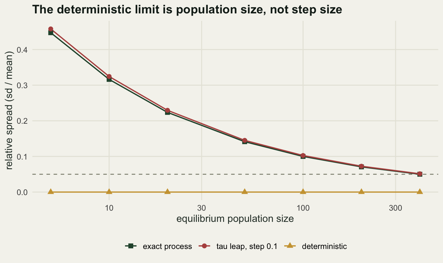
A nonlinear system, where the mean stops being free
Everything above rests on a model whose propensities are linear in the state, and that is exactly why the mean came out free. A real ecological model rarely has that courtesy. Add density dependence and the death propensity becomes quadratic, and the argument that the leap’s expected change equals the true expected change collapses, because the expectation of a square is not the square of the expectation.
So here is the same measurement on a logistic birth-death process with a trickle of immigration to keep it off the absorbing state at zero: births at rate imm2 + b0 * n, deaths at rate d0 * n + cc * n^2. This is still a one-step birth-death chain, so its exact stationary distribution follows from the standard product recursion and needs no simulation either.
imm2 <- 1; b0 <- 1.2; d0 <- 0.2; cc <- 0.01
up_n <- function(n) imm2 + b0 * n
dn_n <- function(n) d0 * n + cc * n * n
nmax_n <- 260
lrat <- c(0, log(up_n(0:(nmax_n - 1))) - log(dn_n(1:nmax_n)))
lp <- cumsum(lrat); lp <- lp - max(lp)
exact_n <- exp(lp); exact_n <- exact_n / sum(exact_n)
mom_exact <- moments_of(exact_n)
ode_eq <- ((b0 - d0) + sqrt((b0 - d0)^2 + 4 * cc * imm2)) / (2 * cc)
print(round(c(exact_mean = mom_exact[["mean"]],
              exact_variance = mom_exact[["variance"]],
              ode_equilibrium = ode_eq,
              state_space_top = nmax_n), 4))
exact_mean exact_variance ode_equilibrium state_space_top
99.7992 120.0418 100.9902 260.0000 taus_n <- 10^seq(log10(0.002), log10(0.2), length.out = 8)
nl <- as.data.frame(t(sapply(taus_n, function(tau) {
ps <- stat_dist(leap_matrix(up_n, dn_n, tau, nmax_n))
mo <- moments_of(ps)
c(tau = tau,
mean_err = abs(mo[["mean"]] - mom_exact[["mean"]]) / mom_exact[["mean"]],
var_err = abs(mo[["variance"]] - mom_exact[["variance"]]) / mom_exact[["variance"]],
tv = tv_dist(ps, exact_n))
})))
print(signif(nl, 4)) tau mean_err var_err tv
1 0.002000 1.231e-05 0.001019 0.0002545
2 0.003861 2.379e-05 0.001970 0.0004916
3 0.007455 4.602e-05 0.003811 0.0009501
4 0.014390 8.919e-05 0.007384 0.0018380
5 0.027790 1.734e-04 0.014360 0.0035620
6 0.053650 3.396e-04 0.028110 0.0069270
7 0.103600 6.743e-04 0.055800 0.0135700
8 0.200000 1.378e-03 0.113900 0.0269500nl_slopes <- c(mean = unname(coef(lm(log(nl$mean_err) ~ log(nl$tau)))[2]),
variance = unname(coef(lm(log(nl$var_err) ~ log(nl$tau)))[2]),
total_variation = unname(coef(lm(log(nl$tv) ~ log(nl$tau)))[2]))
print(round(nl_slopes, 4)) mean variance total_variation
1.0207 1.0205 1.0106 nl_pct <- c(mean_pct_big_step = 100 * nl$mean_err[8],
var_pct_big_step = 100 * nl$var_err[8],
var_over_mean = nl$var_err[8] / nl$mean_err[8],
ode_gap_pct = 100 * (ode_eq - mom_exact[["mean"]]) / ode_eq)
print(signif(nl_pct, 4))mean_pct_big_step var_pct_big_step var_over_mean ode_gap_pct
0.1378 11.3900 82.6900 1.1790 The mean now has an error, and it is a genuine first order error rather than a noise floor: the fitted exponent is 1.0207, alongside 1.0205 for the variance and 1.0106 for the total variation distance. So the linear model’s free lunch really was a special case, and the honest statement is that the leap is first order in everything.
The size of the errors is still wildly unequal, though. At the largest step tested, 0.2, the mean is off by 0.1378 per cent and the variance by 11.39 per cent, a ratio of about 82.69. The general lesson survives the loss of the special case: a step chosen by checking the mean will be roughly two orders of magnitude too coarse for the variance.
There is a second thing in that output worth pointing at. The deterministic equilibrium of this system is 100.9902, while the exact stochastic mean is 99.7992, lower by 1.179 per cent. Density dependence plus noise moves the mean away from the deterministic equilibrium, and the stationary variance of 120.0418 is larger than the mean of 99.7992, so this population is overdispersed relative to Poisson. No choice of tau repairs either of those, because neither is a leaping error.
What to take away
The measurements say three things that do not sit comfortably together. The negative-count crash, which is the failure mode everyone codes a guard for, is a small-population problem: 60.5 per cent of chains at an equilibrium of five with a step of 0.5, and zero out of 400 chains at an equilibrium of eighty at every step tested. The accuracy problem runs the other way, because the standard leap condition at a fixed tolerance grants a step proportional to the population and therefore delivers a variance error that grows with it. And the cheapest diagnostic anyone reaches for, checking that the mean comes out right, is almost useless: in the linear model the mean carries no leaping error at all, only whatever the guard puts there, and in the nonlinear one it is about 82.69 times more accurate than the variance at the same step.
If you are going to leap, check the quantity you are running the model to get. Simulate a small version of your system at two step sizes differing by a factor of four, compare the variance or the extinction probability or whatever the output actually is, and keep halving until it stops moving. That measures the thing you care about, which the leap condition does not.
Here is the honest limit. Every number here comes from two systems chosen because their exact answers are available in closed form or from a one-dimensional recursion, and both are single-species birth-death chains with one relaxation timescale. A real model with several coupled nonlinear reactions, stiff rate constants or a slow-fast structure can behave considerably worse, and the transition-matrix trick that let me measure errors without Monte Carlo noise does not extend to it. The leap condition is a heuristic and not a bound: nothing here proves an error for any system, it only measures one for these. Treat the numbers as a best case and calibrate your own step against your own output.
References
Gillespie DT 1977 The Journal of Physical Chemistry 81(25):2340-2361 (10.1021/j100540a008)
Gillespie DT 2001 The Journal of Chemical Physics 115(4):1716-1733 (10.1063/1.1378322)
Rathinam M, Petzold LR, Cao Y, Gillespie DT 2003 The Journal of Chemical Physics 119(24):12784-12794 (10.1063/1.1627296)
Cao Y, Gillespie DT, Petzold LR 2005 The Journal of Chemical Physics 123(5):054104 (10.1063/1.1992473)
Cao Y, Gillespie DT, Petzold LR 2006 The Journal of Chemical Physics 124(4):044109 (10.1063/1.2159468)
Kurtz TG 1970 Journal of Applied Probability 7(1):49-58 (10.2307/3212147)
MacArthur RH, Wilson EO 1967 The Theory of Island Biogeography (ISBN 978-0-691-08836-5)