library(ggplot2)

te_pal <- list(forest = "#275139", green = "#2f8f63", sage = "#93a87f",
               clay = "#b5534e", gold = "#cda23f", line = "#dad9ca",
               ink = "#16241d", paper = "#f5f4ee")

fmt <- function(x, digits = 4) formatC(x, format = "f", digits = digits)

theme_te <- function() {
  theme_minimal(base_size = 12) +
    theme(panel.grid.minor = element_blank(),
          panel.grid.major = element_line(colour = "#e7e6dc"),
          plot.background = element_rect(fill = "#f5f4ee", colour = NA),
          panel.background = element_rect(fill = "#f5f4ee", colour = NA),
          plot.title = element_text(face = "bold", colour = te_pal$ink),
          axis.title = element_text(colour = "#2c3a31"),
          legend.position = "bottom")
}Checking a stochastic simulation
R
stochastic simulation
model checking
ecology tutorial
Four measured checks on a stochastic ecological simulation in R: replicate count, sampler validation, survivorship bias in the output, and seed handling.
The meeting ran to a single slide. A consultant had built a stochastic population model for a reintroduced population, run it a hundred times, and reported that three of the hundred runs went extinct inside twenty years. The room treated three per cent as the answer, and the discussion moved on to whether three per cent was acceptable.
Nobody asked the question that decides whether the number means anything: how far would that three per cent move if the same code were run again with a different seed. A regression gives you residuals to look at and a standard error to argue with. A simulation gives you whatever you told it to print, at whatever precision you happened to buy, and it prints it just as confidently when the sampler is wrong.
So the checks have to be built on purpose. This post builds four of them, and each one is a measurement against something known rather than an opinion. The first asks how many replicates the reported quantity actually needs, and finds that the answer depends on which quantity by a factor of well over a hundred. The second asks whether the sampler simulates the model it claims to, using a case with a closed form answer, then feeds it two deliberately broken samplers to see whether the check fires. The third asks what happens to an average when some of the runs have already ended. The fourth asks what a seed does, and what happens when two cells of a design share one. Two of the four came out differently from the way they were planned and both are kept as measured: a high quantile turned out to cost a few times a mean rather than orders of magnitude more, and a shared seed between two cells turned out to improve the comparison rather than fake it.
Everything below is base R plus ggplot2. The Gillespie sampler is fifteen lines of loop, the exact answers are two closed form expressions, and the whole post knits in well under a minute with twelve thousand replicates in the reference study. The sampler itself is built from first principles in the Gillespie algorithm from scratch, the price of approximating it is measured in tau leaping and the cost of a bigger step, and the exact extinction time results used here as the truth are derived in mean time to extinction, exactly. This post assumes those and reuses their machinery compactly.
The process, and what is known about it exactly
Three of the four checks run on the same model: a linear birth and death process. Every individual gives birth at rate lam and dies at rate mu independently of every other, so with n individuals alive the total event rate is (lam + mu) * n and the next event is a birth with probability lam / (lam + mu). Zero is absorbing. This is the simplest model in population biology that goes extinct on its own, and one of the few whose extinction time distribution is written down in closed form.
bd_run <- function(n0, lam, mu, t_max = 60) {
  cap <- 512L
  times <- numeric(cap); states <- integer(cap)
  times[1] <- 0; states[1] <- n0
  k <- 1L; n <- n0; tnow <- 0
  p_birth <- lam / (lam + mu)
  while (n > 0L && tnow < t_max) {
    tnow <- tnow + rexp(1, (lam + mu) * n)
    if (tnow >= t_max) break
    n <- n + if (runif(1) < p_birth) 1L else -1L
    k <- k + 1L
    if (k > cap) {
      cap <- 2L * cap
      times <- c(times, numeric(cap / 2)); states <- c(states, integer(cap / 2))
    }
    times[k] <- tnow; states[k] <- n
  }
  list(times = times[1:k], states = states[1:k],
       t_ext = if (n == 0L) times[k] else Inf)
}

bd_study <- function(nrep, n0, lam, mu, grid) {
  tex <- numeric(nrep); traj <- matrix(0L, nrep, length(grid))
  for (i in seq_len(nrep)) {
    r <- bd_run(n0, lam, mu)
    tex[i] <- r$t_ext
    traj[i, ] <- r$states[findInterval(grid, r$times)]
  }
  list(tex = tex, traj = traj)
}
The loop is the standard direct method. Draw the waiting time from an exponential whose rate is the total propensity, advance the clock, then decide which event happened and update the state. The order of those three steps is the whole content of the algorithm, and check two is about what happens when the order is wrong.
bd_study keeps two things per replicate: the extinction time, and the population size read off on a fixed time grid. findInterval returns, for each grid time, the index of the last event at or before it, so the state recorded at a grid point is the state the process was in at that moment, which is what check three needs.
bd_cdf <- function(tt, n0, lam, mu) {
  d <- mu - lam; u <- exp(-d * tt)
  (mu * (1 - u) / (mu - lam * u))^n0
}
bd_pdf <- function(tt, n0, lam, mu) {
  d <- mu - lam; u <- exp(-d * tt)
  al <- mu * (1 - u) / (mu - lam * u)
  n0 * al^(n0 - 1) * mu * d^2 * u / (mu - lam * u)^2
}

n_start <- 10L; lam_bd <- 0.5; mu_bd <- 1.0; horizon <- 1.5
ex_mean <- integrate(function(z) 1 - bd_cdf(z, n_start, lam_bd, mu_bd), 0, Inf)$value
ex_m2 <- 2 * integrate(function(z) z * (1 - bd_cdf(z, n_start, lam_bd, mu_bd)), 0, Inf)$value
ex_sd <- sqrt(ex_m2 - ex_mean^2)
ex_q95 <- uniroot(function(z) bd_cdf(z, n_start, lam_bd, mu_bd) - 0.95, c(0.1, 80))$root
ex_tail <- bd_cdf(horizon, n_start, lam_bd, mu_bd)
ex_f95 <- bd_pdf(ex_q95, n_start, lam_bd, mu_bd)
print(c(n_start = n_start, birth_rate = lam_bd, death_rate = mu_bd,
        horizon = horizon))
n_start birth_rate death_rate horizon
10.0 0.5 1.0 1.5 print(round(c(mean = ex_mean, sd = ex_sd, q95 = ex_q95, p_tail = ex_tail,
density_at_q95 = ex_f95), 4)) mean sd q95 p_tail density_at_q95
4.6402 2.3722 9.1746 0.0247 0.0246 For a single ancestor the probability of extinction by time t is that bracketed expression, and because the lines of descent from the 10 starting individuals are independent, the probability that all of them are gone is that expression to the power 10. Differentiating gives the density, which check one needs for the quantile.
With a birth rate of 0.5 against a death rate of 1.0 this population is doomed: extinction happens with probability one. The mean time it takes is 4.6402, the standard deviation across runs is 2.3722, the 95th percentile is 9.1746, and the probability that the population is gone within 1.5 time units is 0.0247. Those four numbers are the truth for the rest of the post.
n_ref <- 12000L
tgrid <- seq(0, 8, by = 0.25)
set.seed(20260728)
ref <- bd_study(n_ref, n_start, lam_bd, mu_bd, tgrid)
tex <- ref$tex
print(c(reference_runs = n_ref, censored = sum(!is.finite(tex)),
        grid_points = length(tgrid), grid_max = max(tgrid),
        net_rate = mu_bd - lam_bd))
reference_runs censored grid_points grid_max net_rate
12000.0 0.0 33.0 8.0 0.5 print(round(c(mean = mean(tex), sd = sd(tex),
q95 = quantile(tex, 0.95, names = FALSE),
p_tail = mean(tex <= horizon)), 4)) mean sd q95 p_tail
4.6592 2.3901 9.2588 0.0242 12000 runs, none of them still going at the safety cap inside bd_run. The estimated mean is 4.6592 against a true 4.6402, the estimated standard deviation is 2.3901 against 2.3722, the estimated 95th percentile is 9.2588 against 9.1746, and the estimated tail probability is 0.0242 against 0.0247. Each estimate is close, none is exact, and the four are not equally close. That unevenness is the subject of the next section. The same runs are the raw material for check three, because each one carries its population size on the grid out to time 8.
Check one: how many replicates the reported number needs
Monte Carlo error is not a matter of taste. It is a standard error, it has a formula, and it shrinks as one over the square root of the number of replicates for any summary that behaves like an average. What changes between summaries is the constant in front of that square root. For a mean, the relative standard error is the coefficient of variation divided by the square root of the replicate count. For a sample proportion it is the square root of (1 - p) / (p * n), which blows up as p gets small. For a quantile it is sqrt(p * (1 - p) / n) divided by the density at that quantile and again by the quantile itself, and the density is a quantity most people never think about when they report a 95th percentile.
target_rse <- 0.05
rse_mean <- function(nn) (ex_sd / ex_mean) / sqrt(nn)
rse_q95 <- function(nn) sqrt(0.95 * 0.05 / nn) / (ex_f95 * ex_q95)
rse_tail <- function(nn) sqrt((1 - ex_tail) / (ex_tail * nn))

n_need <- c(mean = (ex_sd / ex_mean / target_rse)^2,
            q95 = 0.95 * 0.05 / (ex_f95 * ex_q95 * target_rse)^2,
            p_tail = (1 - ex_tail) / (ex_tail * target_rse^2))
print(round(n_need, 0))
mean q95 p_tail
105 374 15767 print(round(c(tail_over_mean = n_need[["p_tail"]] / n_need[["mean"]],
q95_over_mean = n_need[["q95"]] / n_need[["mean"]]), 2))tail_over_mean q95_over_mean
150.82 3.58 To pin the mean extinction time to a relative standard error of 0.05 takes 105 replicates; the 95th percentile at the same relative precision takes 374, and the probability of extinction within 1.5 time units takes 15767.
The gap between the first and the third is a factor of 150.82, and it is arithmetic rather than a subtlety of the model: a rare event that happens in a fraction 0.0247 of runs carries information only in the runs where it happens, so a study of a hundred runs contains fewer than three informative replicates no matter how long each one took to compute.
The gap between the first and the second came out against expectation. A high quantile is usually described as expensive, and it is more expensive than a mean here, but only by a factor of 3.58. The reason is the density at the quantile, 0.0246 per time unit, small in absolute terms but compared against a quantile of 9.1746 time units, and it is the product of the two that sets the relative precision. For a heavier right tail the same calculation comes out much worse. The lesson is not that quantiles are cheap; it is that the cost is computable in advance.
batch_sizes <- c(20L, 40L, 80L, 160L)
n_split <- 8L
set.seed(46512300)
meas <- NULL
for (nn in batch_sizes) {
  nb <- n_ref %/% nn
  acc <- matrix(0, n_split, 3)
  for (s in seq_len(n_split)) {
    mm <- matrix(tex[sample.int(n_ref)][seq_len(nb * nn)], nn, nb)
    bm <- colMeans(mm)
    bq <- apply(mm, 2, quantile, probs = 0.95, names = FALSE)
    bp <- colMeans(mm <= horizon)
    acc[s, ] <- c(sd(bm) / mean(bm), sd(bq) / mean(bq), sd(bp) / mean(bp))
  }
  meas <- rbind(meas, data.frame(n = nn, batches = nb,
    measured_mean = mean(acc[, 1]), exact_mean = rse_mean(nn),
    measured_q95 = mean(acc[, 2]), exact_q95 = rse_q95(nn),
    measured_tail = mean(acc[, 3]), exact_tail = rse_tail(nn)))
}
print(round(meas, 4), row.names = FALSE)
n batches measured_mean exact_mean measured_q95 exact_q95 measured_tail
20 600 0.1139 0.1143 0.1906 0.2164 1.4273
40 300 0.0787 0.0808 0.1434 0.1530 0.9899
80 150 0.0571 0.0572 0.1062 0.1082 0.7151
160 75 0.0417 0.0404 0.0788 0.0765 0.4808
exact_tail
1.4039
0.9927
0.7019
0.4963print(c(splits_per_size = n_split, target_rse = target_rse))splits_per_size target_rse
8.00 0.05 Those formulas are worth checking rather than trusting. The reference set is cut into disjoint batches of 20, 40, 80 and 160 runs, each batch is treated as a small independent study, and the spread across batches is the Monte Carlo standard error measured directly; the cut is repeated over 8 random shuffles and averaged, because the spread of a few dozen batches is itself noisy.
At 80 replicates per batch the measured relative standard error of the mean is 0.0571 against a predicted 0.0572, and the measured tail figure is 0.7151 against 0.7019. The quantile is the one place where small sample behaviour shows: at 20 replicates the measured value is 0.1906 while the large sample formula says 0.2164, because a 95th percentile computed from 20 numbers is an interpolation between the two largest of them and that is not the estimator the asymptotic formula describes. By 160 replicates the measured value is 0.0788 against a predicted 0.0765.
set.seed(90210777)
n_small <- 100L; n_paper <- 2000L
p_hat_100 <- rbinom(n_paper, n_small, ex_tail) / n_small
print(c(n_small = n_small, studies = n_paper))
n_small studies
100 2000 print(round(c(lower = quantile(p_hat_100, 0.025, names = FALSE),
upper = quantile(p_hat_100, 0.975, names = FALSE),
frac_zero = mean(p_hat_100 == 0), true_value = ex_tail), 4)) lower upper frac_zero true_value
0.0000 0.0600 0.0745 0.0247 This is the consultant’s slide, simulated 2000 times: each study runs the model 100 times and reports the fraction that went extinct within the horizon, whose true value is 0.0247. Ninety five per cent of what those studies report falls between 0.0000 and 0.0600, and a fraction 0.0745 of them report the probability as exactly zero.
An interval that runs from nothing to more than twice the truth is not a result. It is a coin flip dressed as a number, and it costs nothing to detect in advance: the required replicate count can be evaluated before any simulation is run, from a rough guess at the probability. Get the guess wrong by a factor of two and the count is still right to within the same factor, which is all the guidance a design needs.
xs <- 10^seq(log10(20), log10(40000), length.out = 120)
lv <- c("mean", "95th percentile", "P(extinct by 1.5)")
lin <- data.frame(n = xs, rse = c(rse_mean(xs), rse_q95(xs), rse_tail(xs)),
                  what = factor(rep(lv, each = length(xs)), lv))
pts <- data.frame(n = meas$n, rse = c(meas$measured_mean, meas$measured_q95,
                                      meas$measured_tail),
                  what = factor(rep(lv, each = nrow(meas)), lv))
cols <- c(te_pal$green, te_pal$gold, te_pal$clay); names(cols) <- lv

ggplot(lin, aes(n, rse, colour = what)) +
  geom_hline(yintercept = target_rse, linetype = "22", colour = te_pal$ink) +
  geom_line(linewidth = 0.9) +
  geom_point(data = pts, size = 2.4, shape = 16) +
  scale_x_log10(breaks = c(20, 100, 1000, 10000, 40000),
                labels = c("20", "100", "1000", "10000", "40000")) +
  scale_y_log10(breaks = c(0.01, 0.05, 0.2, 1, 3),
                labels = c("0.01", "0.05", "0.2", "1", "3")) +
  scale_colour_manual(values = cols, name = NULL) +
  labs(title = "Monte Carlo error of three summaries of one simulation",
       x = "replicates in the study", y = "relative standard error") +
  theme_te()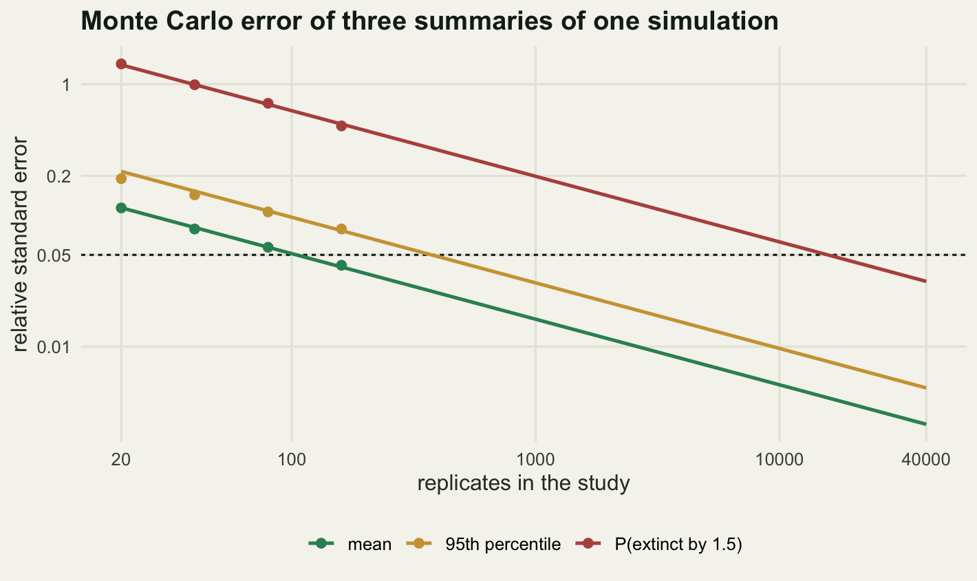
On a log scale the one over root n law is a straight line of slope minus one half, and all three summaries lie on lines of that slope. That is what licenses extrapolation: having measured the error at 160 replicates you can read off what it will be at ten thousand without running ten thousand. The interesting part is the vertical spacing, because the three lines never meet. Whatever budget you have, the tail probability is between one and two orders of magnitude less precise than the mean computed from the very same runs, and a study that reports both usually gives them the same number of decimal places.
Check two: does the sampler sample the model
A sampler with a bug in it still produces output, and the output still looks like a stochastic process. The only real check is a case where the answer is known in advance, so the check has to be built on a model chosen for being solvable rather than interesting. The immigration and death process is the standard choice: individuals arrive from outside at a constant rate imm regardless of how many are present, each present individual dies at rate dth, and the stationary distribution of the population size is Poisson with mean imm / dth, exactly, with no free parameters left to fit.
im_run <- function(a, mu, t_end, mode = "correct") {
  n <- 0L; tnow <- 0; rate_prev <- a; n_ev <- 0L
  repeat {
    rate <- a + mu * n
    is_birth <- runif(1) < a / rate
    dt <- switch(mode,
      correct     = rexp(1, rate),
      chosen_rate = rexp(1, if (is_birth) a else mu * n),
      stale_rate  = rexp(1, rate_prev))
    tnow <- tnow + dt
    if (tnow > t_end) break
    n <- n + if (is_birth) 1L else -1L
    rate_prev <- rate; n_ev <- n_ev + 1L
  }
  c(n, n_ev)
}

im_study <- function(k, a, mu, t_end, mode) {
  out <- matrix(0L, k, 2)
  for (i in seq_len(k)) out[i, ] <- im_run(a, mu, t_end, mode)
  out
}
One function, three samplers. In correct mode the waiting time is drawn from the total propensity, which is what the algorithm requires. In chosen_rate mode the reaction is picked first, correctly, and then the waiting time is drawn from that reaction’s own rate instead of the total. This is the bug people write when they reason that the next immigration happens after an Exp(a) wait: true in isolation, wrong in competition, because two clocks are running and only the smaller counts. In stale_rate mode the waiting time comes from the propensity of the previous state, which is the bug people write when they hoist the propensity calculation out of the loop or update the state before recomputing it.
imm <- 2; dth <- 1; t_end <- 12; n_run <- 1500L
set.seed(80153962)
run_ok <- im_study(n_run, imm, dth, t_end, "correct")
run_st <- im_study(n_run, imm, dth, t_end, "stale_rate")
run_ch <- im_study(n_run, imm, dth, t_end, "chosen_rate")
run_ch4 <- im_study(n_run, 4, dth, t_end, "chosen_rate")
print(c(immigration = imm, death = dth, t_end = t_end, replicates = n_run,
        poisson_target = imm / dth))
immigration death t_end replicates poisson_target
2 1 12 1500 2 print(round(c(mean_correct = mean(run_ok[, 1]), mean_stale = mean(run_st[, 1]),
mean_chosen = mean(run_ch[, 1]),
mean_chosen_lam4 = mean(run_ch4[, 1])), 4)) mean_correct mean_stale mean_chosen mean_chosen_lam4
1.9820 2.1387 2.1640 3.9540 Each sampler is run 1500 times from an empty population out to time 12, and the population size at the end of each run is recorded. With a death rate of 1 the relaxation time is one time unit, so that end point sits far inside the stationary regime, and with an immigration rate of 2 the target is Poisson with mean 2. The correct sampler averages 1.9820, the stale rate sampler 2.1387 and the chosen rate sampler 2.1640. The fourth run is the chosen rate bug with the immigration rate raised to four, which matters shortly.
gof <- function(x, lam_p, n_cell, k) {
  pex <- c(dpois(0:(n_cell - 2L), lam_p), 1 - ppois(n_cell - 2L, lam_p))
  obs <- tabulate(pmin(x, n_cell - 1L) + 1L, n_cell)
  exp_c <- k * pex
  list(x2 = sum((obs - exp_c)^2 / exp_c), obs = obs, exp = exp_c,
       resid = (obs - exp_c) / sqrt(exp_c))
}

n_cell2 <- 7L; n_cell4 <- 10L
g_ok <- gof(run_ok[, 1], 2, n_cell2, n_run)
g_st <- gof(run_st[, 1], 2, n_cell2, n_run)
g_ch <- gof(run_ch[, 1], 2, n_cell2, n_run)
g_ch4 <- gof(run_ch4[, 1], 4, n_cell4, n_run)
print(round(c(correct = g_ok$x2, stale_rate = g_st$x2, chosen_rate = g_ch$x2,
              chosen_rate_lam4 = g_ch4$x2), 3))
correct stale_rate chosen_rate chosen_rate_lam4
2.369 22.699 66.181 12.032 print(c(cells_lam2 = n_cell2, cells_lam4 = n_cell4,
df_lam2 = n_cell2 - 1L, df_lam4 = n_cell4 - 1L))cells_lam2 cells_lam4 df_lam2 df_lam4
7 10 6 9 The counts are binned into 7 cells (population sizes zero to five, plus a cell for six and above), the expected cell probabilities come from the Poisson with no parameters estimated, and the statistic is the usual sum of squared standardised deviations; because nothing was fitted, the reference distribution has 6 degrees of freedom rather than fewer. The statistic is 2.369 for the correct sampler, 22.699 for the stale rate bug and 66.181 for the chosen rate bug. Two of those look damning and one looks fine, but a statistic is only as good as the distribution it is compared against.
set.seed(70410855)
n_null <- 4000L
null2 <- numeric(n_null); null4 <- numeric(n_null)
for (b in seq_len(n_null)) {
  null2[b] <- gof(rpois(n_run, 2), 2, n_cell2, n_run)$x2
  null4[b] <- gof(rpois(n_run, 4), 4, n_cell4, n_run)$x2
}
print(round(c(null_draws = n_null, null_mean = mean(null2),
              null_q95 = quantile(null2, 0.95, names = FALSE),
              chisq_q95 = qchisq(0.95, n_cell2 - 1),
              reject_rate = mean(null2 >= qchisq(0.95, n_cell2 - 1))), 4))
null_draws null_mean null_q95 chisq_q95 reject_rate
4000.0000 6.0593 12.8097 12.5916 0.0545 print(round(c(null4_mean = mean(null4), null4_q95 = quantile(null4, 0.95, names = FALSE),
chisq4_q95 = qchisq(0.95, n_cell4 - 1),
reject_rate4 = mean(null4 >= qchisq(0.95, n_cell4 - 1))), 4)) null4_mean null4_q95 chisq4_q95 reject_rate4
9.0756 17.0009 16.9190 0.0512 print(round(c(p_correct = mean(null2 >= g_ok$x2), p_stale = mean(null2 >= g_st$x2),
p_chosen = mean(null2 >= g_ch$x2),
p_chosen_lam4 = mean(null4 >= g_ch4$x2)), 4)) p_correct p_stale p_chosen p_chosen_lam4
0.8728 0.0015 0.0000 0.2112 Calibrating the null costs one line: draw 1500 numbers straight from the Poisson the sampler should be producing, compute the statistic, and repeat 4000 times. That gives the distribution of the statistic when nothing is wrong, with no appeal to asymptotics. The mean of the calibrated null is 6.0593 against a nominal 6, and its 95th percentile is 12.8097 against a chi-squared value of 12.5916. Using the chi-squared critical value rejects a fraction 0.0545 of correct samples rather than the nominal five per cent, and for the wider 10 cell version the figure is 0.0512. With 4000 calibration draws the Monte Carlo error on those fractions is a few thousandths, so both are consistent with the nominal level. The approximation holds here, and it is still worth the one line that showed it does, because it holds only when the expected cell counts are large; the version of this check written with twenty cells and two hundred replicates is a different story.
Against the calibrated null the correct sampler sits at 0.8728, the stale rate bug at 0.0015 and the chosen rate bug at 0.0000. The check fires on both bugs. A check that has never fired on a known bug is not a check, and this one has now fired twice.
res_tab <- rbind(correct = g_ok$resid, stale_rate = g_st$resid, chosen_rate = g_ch$resid)
colnames(res_tab) <- c(0:5, "6+")
print(round(res_tab, 3))
0 1 2 3 4 5 6+
correct 1.053 -0.695 0.496 -0.284 -0.631 -0.018 0.232
stale_rate -3.509 -1.042 1.439 0.749 1.175 2.292 -0.170
chosen_rate -7.300 2.233 0.397 1.965 1.432 -0.562 1.235print(round(c(share_cell0_chosen = g_ch$resid[1]^2 / g_ch$x2,
share_cell0_stale = g_st$resid[1]^2 / g_st$x2,
share_cell0_chosen_lam4 = g_ch4$resid[1]^2 / g_ch4$x2), 4)) share_cell0_chosen share_cell0_stale share_cell0_chosen_lam4
0.8051 0.5426 0.3318 sname <- c("correct", "stale rate", "chosen rate")
rdat <- data.frame(cell = 0:(n_cell2 - 1L), r = as.vector(t(res_tab)),
sampler = factor(rep(sname, each = n_cell2), sname))
scol <- c(te_pal$green, te_pal$gold, te_pal$clay); names(scol) <- sname
ggplot(rdat, aes(cell, r, colour = sampler, shape = sampler)) +
geom_hline(yintercept = 0, colour = te_pal$ink, linewidth = 0.4) +
geom_hline(yintercept = c(-2, 2), linetype = "22", colour = "#8a8a7a") +
geom_line(linewidth = 0.7) +
geom_point(size = 2.6) +
scale_colour_manual(values = scol, name = NULL) +
scale_shape_manual(values = c(16, 17, 15), name = NULL) +
scale_x_continuous(breaks = 0:6, labels = c(0:5, "6+")) +
labs(title = "Where each sampler disagrees with Poisson(2)",
x = "population size cell", y = "standardised residual") +
theme_te()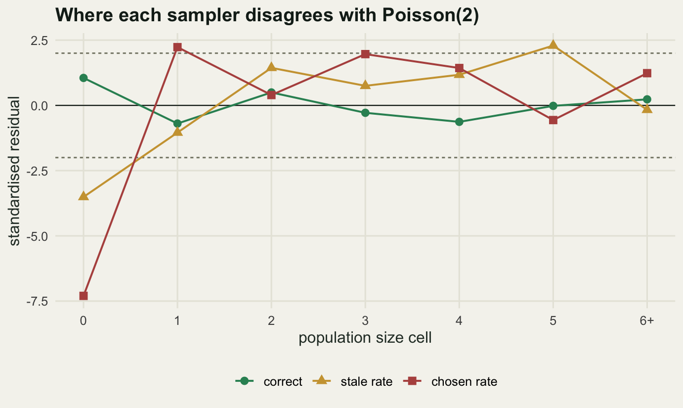
The residuals say where the disagreement lives, and the two bugs disagree in different places. The chosen rate bug puts a residual of -7.300 in the cell for an empty population and stays inside plus or minus two and a half everywhere else, so that single cell accounts for a fraction 0.8051 of its statistic. The stale rate bug also misses low at an empty population, at -3.509, but only 0.5426 of its statistic is there and the rest is spread across the upper cells. That concentration turns the section around.
bt <- data.frame(poisson_mean = c(2, 4),
                 p_zero = dpois(0, c(2, 4)),
                 predicted_p_zero = 0.5 * dpois(0, c(2, 4)) / (1 - 0.5 * dpois(0, c(2, 4))),
                 predicted_mean = c(2, 4) / (1 - 0.5 * dpois(0, c(2, 4))),
                 observed_p_zero = c(g_ch$obs[1], g_ch4$obs[1]) / n_run)
print(round(bt, 4), row.names = FALSE)
poisson_mean p_zero predicted_p_zero predicted_mean observed_p_zero
2 0.1353 0.0726 2.1452 0.0660
4 0.0183 0.0092 4.0370 0.0113print(round(c(x2_lam2 = g_ch$x2, x2_lam4 = g_ch4$x2,
crit_lam2 = qchisq(0.95, n_cell2 - 1),
crit_lam4 = qchisq(0.95, n_cell4 - 1),
p_lam4 = mean(null4 >= g_ch4$x2)), 4)) x2_lam2 x2_lam4 crit_lam2 crit_lam4 p_lam4
66.1806 12.0320 12.5916 16.9190 0.2112 Under the chosen rate bug, a state with two competing reactions is held for a waiting time drawn from one of the two rates, picked with the correct probability. The average of that mixture is exactly twice the correct holding time in every state where both reactions are possible, and a uniform doubling cancels out of a stationary distribution: the sampler runs at half speed and occupies the states in the correct proportions. The single exception is the empty population, where only immigration can happen, so there is nothing to average and the holding time is right. That state alone is held for half as long relative to the others as it should be, which halves its weight and inflates the rest by the normalising constant.
That prediction is arithmetic with no fitting in it. For a Poisson mean of two the empty state should carry 0.1353 of the mass and the bug should reduce it to 0.0726; the sampler delivered 0.0660. The predicted mean under the bug is 2.1452, the sampler 2.1640.
Now push the immigration rate to four. The empty state carries only 0.0183 of the mass, so halving its weight changes the distribution by very little: the predicted probability of an empty population drops to 0.0092 and the predicted mean rises only to 4.0370. The statistic on 1500 replicates comes out at 12.032 against a critical value of 16.919, which is a p value of 0.2112. The check passes.
The same bug, the same code, the same number of replicates, and the goodness of fit test catches it at one parameter setting and clears it at another. What decided the outcome was how much probability mass happened to sit in the one state where the bug bites. Choosing the parameters of a test case for convenience is choosing the power of the check.
ev_exact <- function(a, mu, te) 2 * a * te - (a / mu) * (1 - exp(-mu * te))
print(round(c(exact = ev_exact(2, 1, t_end), correct = mean(run_ok[, 2]),
              se_correct = sd(run_ok[, 2]) / sqrt(n_run),
              stale_rate = mean(run_st[, 2]),
              se_stale = sd(run_st[, 2]) / sqrt(n_run),
              chosen_rate = mean(run_ch[, 2])), 3))
exact correct se_correct stale_rate se_stale chosen_rate
46.000 45.893 0.248 45.189 0.251 24.689 print(round(c(exact_lam4 = ev_exact(4, 1, t_end),
chosen_rate_lam4 = mean(run_ch4[, 2]),
se = sd(run_ch4[, 2]) / sqrt(n_run),
standard_errors_off = (ev_exact(4, 1, t_end) - mean(run_ch4[, 2])) /
(sd(run_ch4[, 2]) / sqrt(n_run))), 3)) exact_lam4 chosen_rate_lam4 se standard_errors_off
92.000 45.415 0.251 185.273 There is a second exact quantity available and it costs nothing to record: the number of events per run. The expected number in a window of length t_end is the integral of the total propensity over it, which here has a closed form. The correct sampler should average 46.000 events and delivers 45.893, with a Monte Carlo standard error of 0.248. The stale rate sampler delivers 45.189, which is 3.2 standard errors low, so this check sees that bug too, quietly. The chosen rate sampler delivers 24.689 events where it should deliver 46.000, and at the higher immigration rate it delivers 45.415 where it should deliver 92.000: a difference of 185 standard errors, in exactly the setting where the distribution check saw nothing. The two checks differ in how loudly they speak, and the one that shouts about a bug is not the one that shouts about the other. Recording the event count costs one integer per run.
Check three: the runs that are no longer there
Runs that end early are not missing at random. They are missing because of what happened in them, so any average over the runs still going is an average over a sample filtered by the outcome. Ecologists recognise this at once when it happens to marked animals, and then write the simulation version without noticing.
alive <- ref$traj > 0L
n_alive <- colSums(alive)
mean_cond <- colSums(ref$traj) / pmax(n_alive, 1L)
mean_unc <- colMeans(ref$traj)
ex_unc <- n_start * exp(-(mu_bd - lam_bd) * tgrid)
p_surv <- 1 - bd_cdf(tgrid, n_start, lam_bd, mu_bd); p_surv[1] <- 1
ex_cond <- ex_unc / p_surv

sel <- which(tgrid %in% c(2, 4, 6, 8))
print(data.frame(time = tgrid[sel], still_running = n_alive[sel],
                 conditional = round(mean_cond[sel], 3),
                 unconditional = round(mean_unc[sel], 3),
                 exact_cond = round(ex_cond[sel], 3),
                 exact_unc = round(ex_unc[sel], 3),
                 ratio = round(mean_cond[sel] / mean_unc[sel], 3)),
      row.names = FALSE)
time still_running conditional unconditional exact_cond exact_unc ratio
2 11118 3.980 3.688 3.989 3.679 1.079
4 6417 2.550 1.364 2.557 1.353 1.870
6 2762 2.157 0.496 2.185 0.498 4.345
8 1060 2.107 0.186 2.066 0.183 11.321Two averages, same 12000 runs. The conditional one divides the total population by the replicates still running; the unconditional one divides by all 12000, carrying every extinct replicate at its absorbing value of zero. For this process the unconditional mean is available in closed form, as 10 times an exponential decay at rate 0.5 per time unit, because expectations of a linear birth and death process do not care about the absorbing boundary. Dividing by the probability of still being alive gives the exact conditional mean, so both averages can be checked.
At time 4, 6417 of the 12000 runs are still going, and the two means are 2.550 and 1.364, a ratio of 1.870. By time 8 only 1060 runs remain and the two means are 2.107 and 0.186, a ratio of 11.321.
qn <- c("conditional on still running", "unconditional (absorbed at zero)")
cdat <- data.frame(time = tgrid, y = c(mean_cond, mean_unc),
                   quantity = rep(qn, each = length(tgrid)))
ksel <- seq(1, length(tgrid), by = 4)
edat <- data.frame(time = tgrid[ksel], y = c(ex_cond[ksel], ex_unc[ksel]),
                   quantity = rep(qn, each = length(ksel)), src = "exact value")

ggplot(cdat, aes(time, y, colour = quantity)) +
  geom_line(linewidth = 1) +
  geom_point(data = edat, aes(shape = src), size = 2.6, stroke = 0.8, fill = NA) +
  scale_colour_manual(values = setNames(c(te_pal$clay, te_pal$green), qn), name = NULL) +
  scale_shape_manual(values = c(`exact value` = 21), name = NULL) +
  labs(title = "Mean population size, two ways of averaging",
       x = "time", y = "mean population size") +
  guides(colour = guide_legend(nrow = 2, order = 1),
         shape = guide_legend(nrow = 2, order = 2)) +
  theme_te()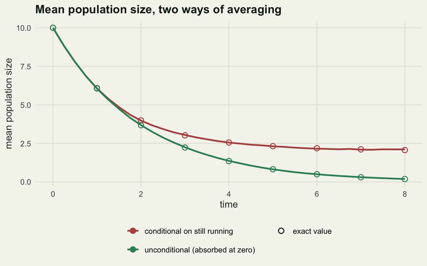
The picture is the reason this matters. The conditional curve flattens: from about time five it sits just above two and stops moving, and if that curve were the only output of the simulation the natural reading would be that the population settles at a small but persistent size. It does no such thing. The unconditional curve decays the whole time, reaching 0.186 at time 8.
What the flat conditional curve describes is the quasi-stationary state: the shape a population takes when you look only at the ones that have not died yet. That is a real and useful quantity, and it answers what a surviving population looks like rather than what a population looks like. The two get confused because the plot looks the same either way.
There are two honest ways to report this and only two. Report the conditional quantity and say what it is conditional on, including the sample size behind it, which at time 8 is 1060 runs rather than 12000. Or report the unconditional quantity with the absorbed runs carried at zero, which is what the exact calculation gives and what a manager asking about expected abundance is asking for. Neither is wrong. Sliding silently from one to the other, as a plotting routine that drops finished runs will do, is what is wrong.
Check four: seeds, streams and what sharing one costs
A seed does one thing: it sets the state of the random number generator, and every subsequent draw comes off one stream in the order the code asks for it. That is simple to state and easy to get wrong in a loop.
one_tex <- function(lam) bd_run(n_start, lam, mu_bd)$t_ext
n_d <- 400L
study_top <- function(lam) vapply(seq_len(n_d), function(i) one_tex(lam), 0)
study_fixed <- function(lam, s) vapply(seq_len(n_d), function(i) { set.seed(s); one_tex(lam) }, 0)
study_cell <- function(lam, base) vapply(seq_len(n_d), function(i) { set.seed(base + i); one_tex(lam) }, 0)

set.seed(20260728)
s_top <- study_top(lam_bd)
s_fix <- study_fixed(lam_bd, 4242)
s_cell <- study_cell(lam_bd, 900000)
seed_tab <- data.frame(
  distinct = c(length(unique(s_top)), length(unique(s_fix)), length(unique(s_cell))),
  est = c(mean(s_top), mean(s_fix), mean(s_cell)),
  spread = c(sd(s_top), sd(s_fix), sd(s_cell)))
seed_tab$mc_se <- seed_tab$spread / sqrt(n_d)
seed_tab$ci_width <- 2 * 1.96 * seed_tab$mc_se
seed_tab$abs_error <- abs(seed_tab$est - ex_mean)
print(round(seed_tab, 4), row.names = FALSE)
distinct est spread mc_se ci_width abs_error
400 4.7931 2.4015 0.1201 0.4707 0.1529
1 4.1296 0.0000 0.0000 0.0000 0.5106
400 4.6204 2.2732 0.1137 0.4455 0.0198print(c(study_replicates = n_d))study_replicates
400 Three seeding patterns, 400 replicates each, all estimating the same mean extinction time whose true value is 4.6402. The first row sets one seed before the loop and lets the stream run: 400 distinct values, an estimate of 4.7931, a Monte Carlo standard error of 0.1201.
The second row sets the same seed at the top of every iteration, so it gives 1 distinct value: every replicate is the same replicate, run 400 times. The estimate is 4.1296, the spread across replicates 0.0000, the standard error 0.0000, and the ninety five per cent interval has width 0.0000. The reported answer is wrong by 0.5106, against a Monte Carlo standard error of 0.1201 for an honest study of the same size, and the interval that would have caught the error has collapsed to a point. This is the failure mode that produces a paper with impossible precision, and it leaves no trace in the output except a suspiciously round interval.
The third row sets a different seed per replicate, derived from the loop index. That pattern gets treated with suspicion, on the grounds that consecutive seeds might produce related streams. It does not here: 400 distinct values, an estimate of 4.6204, a spread of 2.2732 against the true 2.3722, and an error of 0.0198, smaller than the error of the single top level seed in the first row, which is 0.1529. For the Mersenne Twister, consecutive seeds are scattered through the state space and the resulting streams behave as independent at this scale.
lam_hi <- 0.6
cell_a_sh <- study_cell(lam_bd, 700000); cell_b_sh <- study_cell(lam_hi, 700000)
cell_a_of <- study_cell(lam_bd, 100000); cell_b_of <- study_cell(lam_hi, 500000)
pair_tab <- data.frame(correlation = c(cor(cell_a_sh, cell_b_sh),
                                       cor(cell_a_of, cell_b_of)),
  difference = c(mean(cell_b_sh - cell_a_sh), mean(cell_b_of - cell_a_of)),
  se_paired = c(sd(cell_b_sh - cell_a_sh), sd(cell_b_of - cell_a_of)) / sqrt(n_d),
  se_naive = c(sqrt(var(cell_a_sh) + var(cell_b_sh)),
               sqrt(var(cell_a_of) + var(cell_b_of))) / sqrt(n_d))
pair_tab$inflation <- pair_tab$se_naive / pair_tab$se_paired
print(round(pair_tab, 4), row.names = FALSE)
correlation difference se_paired se_naive inflation
0.6065 0.6672 0.1221 0.1877 1.5378
-0.0121 0.6753 0.1977 0.1966 0.9941print(c(birth_rate_cell_a = lam_bd, birth_rate_cell_b = lam_hi))birth_rate_cell_a birth_rate_cell_b
0.5 0.6 The per replicate seed is what makes a single cell of a design reproducible on its own: one awkward replicate of the high birth rate cell can be rerun exactly without touching the rest of the cell or the rest of the grid. The question is what happens when two cells use the same seeds. The first row above is a two cell comparison, birth rate 0.5 against 0.6, where replicate i of both cells starts from the same seed. The second row offsets the seeds so the cells draw from unrelated streams.
Sharing the seeds correlates the cells: the sample correlation between paired replicates is 0.6065, against -0.0121 when the seeds are offset. That is the coupling the usual advice warns about, and the usual conclusion is that it inflates the apparent precision. It does the opposite. The two designs estimate the same difference between cells, 0.6672 with shared seeds and 0.6753 with offset seeds. The standard error of that difference, computed from the paired differences, is 0.1221 for the shared design against 0.1977 for the offset one. Sharing the seeds made the comparison more precise, because the same random numbers drive both cells and the shared noise cancels in the difference. This is the common random numbers trick, a deliberate technique rather than an accident.
The mistake is a different one. Compute the standard error of that difference as though the cells were independent, adding the two variances, and you get 0.1877 for the shared design, overstating the paired value by a factor of 1.5378. For the offset design the two formulas agree, at 0.1966 and 0.1977. So the cost of shared seeds is not fake precision; it is that the analysis has to know the design is paired, and most grid summaries do not.
sn <- c("shared between cells", "offset between cells")
sdat <- data.frame(a = c(cell_a_of, cell_a_sh), b = c(cell_b_of, cell_b_sh),
                   seeds = factor(rep(rev(sn), each = n_d), sn))
ggplot(sdat, aes(a, b, colour = seeds, alpha = seeds)) +
  annotate("segment", x = 0, xend = 16, y = 0, yend = 16, colour = te_pal$ink, linewidth = 0.4) +
  geom_point(size = 1.5) +
  scale_colour_manual(values = setNames(c(te_pal$forest, te_pal$clay), sn), name = NULL,
                      guide = guide_legend(override.aes = list(alpha = 1, size = 2.4))) +
  scale_alpha_manual(values = setNames(c(0.75, 0.3), sn), guide = "none") +
  coord_cartesian(xlim = c(0, 16), ylim = c(0, 20)) +
  labs(title = "Paired replicates in two cells of the same grid",
       x = "extinction time, cell with birth rate 0.5",
       y = "extinction time, cell with birth rate 0.6") +
  theme_te()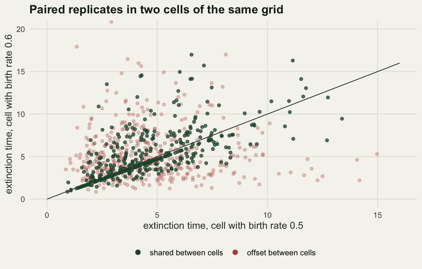
The picture makes the correlation concrete. The shared seed points lie in a band around the diagonal because replicate i in the two cells starts from the same stream and follows a similar path until the different birth rates pull them apart. Read as evidence about the two cells rather than about the seeding, that band would look like a strong biological relationship. It is the same random numbers appearing twice.
set.seed(60606060); ord1_a <- study_top(lam_bd); ord1_b <- study_top(lam_hi)
set.seed(60606060); ord2_b <- study_top(lam_hi); ord2_a <- study_top(lam_bd)
print(round(c(order1_B = mean(ord1_b), order2_B = mean(ord2_b),
              abs_gap = abs(mean(ord2_b) - mean(ord1_b)),
              mc_se_B = sd(ord1_b) / sqrt(n_d)), 4))
order1_B order2_B abs_gap mc_se_B
5.4697 5.1213 0.3484 0.1562 set.seed(60606060); pr1_a <- study_cell(lam_bd, 300000); pr1_b <- study_cell(lam_hi, 400000)
set.seed(60606060); pr2_b <- study_cell(lam_hi, 400000); pr2_a <- study_cell(lam_bd, 300000)
print(c(top_seed_reproducible = identical(ord1_b, ord2_b),
cell_seed_reproducible = identical(pr1_b, pr2_b))) top_seed_reproducible cell_seed_reproducible
FALSE TRUE The last measurement is the one people assume they do not need to make. A seed at the top of the script is supposed to make the study reproducible; it makes the script reproducible, which is not the same claim. Both blocks above start from the same seed and run the same two cells, and the only difference between them is the order. Running the low birth rate cell first gives the high birth rate cell a mean of 5.4697; running that cell first gives 5.1213, a gap of 0.3484 against a Monte Carlo standard error of 0.1562. The two results are not identical, and identical on the raw vectors returns FALSE.
That is what a top level seed buys: rerun the whole file unchanged and you get the same numbers. Add a diagnostic that draws one random number, comment out a cell, reorder two blocks, or run a section interactively before the rest, and every number downstream changes. With per cell seeds the same reordering leaves the results untouched and identical returns TRUE. That is worth more than it sounds, because the reordering usually happens six months later during revision, when nobody remembers that the figure was made before the supplementary analysis rather than after it.
What to take away
Four checks, four measurements. The replicate count needed to report a quantity depends on which quantity: 105 runs for the mean extinction time, 374 for the 95th percentile and 15767 for a tail probability of 0.0247, all at the same relative precision. A hundred run study reporting that tail probability produces something between 0.0000 and 0.0600, and reports exactly zero in a fraction 0.0745 of the studies. A goodness of fit test against an exactly known stationary distribution caught both deliberate bugs at one parameter setting and cleared one of them at another, where an event count check with an exact expectation caught it immediately. Averaging over the runs still going overstated the mean population size by a factor of 11.321 at time 8. A seed set inside the loop collapsed 400 replicates to 1, and a seed set once at the top failed to survive a reordering of the code.
Two of those went against the plan. The 95th percentile cost 3.58 times the mean rather than orders of magnitude, because the density at the quantile is not small once it is expressed relative to the quantile itself. Shared seeds between cells helped the comparison rather than faking it, cutting the standard error of the difference from 0.1977 in the offset design to 0.1221 in the shared one, with the real error being an analysis that ignores the pairing.
The honest limit applies to the whole approach: every check here ran against a model with a closed form answer, and the simulation you actually care about will not have one. What transfers is not the birth and death process but the habit of building the check where the answer is known, which means writing the special case your code can solve exactly (turn off density dependence, set a rate to zero, shrink the landscape to one cell) plus the invariants that survive into the general case: total event counts, conserved individuals, marginal distributions of single components. A sampler that fails on the solvable special case is broken in the general one too, and that is the only direction the argument runs. Nothing here shows that a sampler which passes is correct.
References
Gillespie DT 1977 Journal of Physical Chemistry 81(25):2340-2361 (10.1021/j100540a008)
Gillespie DT 2001 Journal of Chemical Physics 115(4):1716-1733 (10.1063/1.1378322)
Kendall DG 1948 Annals of Mathematical Statistics 19(1):1-15 (10.1214/aoms/1177730285)
Koehler E, Brown E, Haneuse SJ 2009 The American Statistician 63(2):155-162 (10.1198/tast.2009.0030)
Morris TP, White IR, Crowther MJ 2019 Statistics in Medicine 38(11):2074-2102 (10.1002/sim.8086)
Matsumoto M, Nishimura T 1998 ACM Transactions on Modeling and Computer Simulation 8(1):3-30 (10.1145/272991.272995)