library(ggplot2)

te_paper  <- "#f5f4ee"
te_ink    <- "#16241d"
te_body   <- "#2c3a31"
te_forest <- "#275139"
te_rust   <- "#b5534e"
te_gold   <- "#c9b458"
te_line   <- "#dad9ca"

theme_datasheet <- function() {
  theme_minimal(base_size = 12) +
    theme(plot.background  = element_rect(fill = te_paper, colour = NA),
          panel.background = element_rect(fill = te_paper, colour = NA),
          panel.grid.major = element_line(colour = te_line, linewidth = 0.3),
          panel.grid.minor = element_blank(),
          text             = element_text(colour = te_body),
          plot.title       = element_text(colour = te_ink, face = "bold"),
          plot.subtitle    = element_text(colour = te_body),
          axis.text        = element_text(colour = te_body))
}
h2_cols <- c("0.1" = te_rust, "0.2" = te_gold, "0.5" = te_forest)Evolutionary rescue and starting population size
R
evolutionary ecology
quantitative genetics
extinction
simulation
ecology tutorial
Evolutionary rescue in R: a branching process and an individual-based model show even odds need a Gomulkiewicz-Holt minimum of 5 to 15 individuals, not one.
A lake warms by a few degrees over a decade and then stays warm. The copepod that lives in it has a thermal optimum set by the old water, and in the new water the average female no longer replaces herself: each generation is smaller than the last. The copepod has heritable variation in thermal tolerance, so selection starts moving the population towards the new optimum at once. Whether that is enough depends on a race. Adaptation raises mean fitness a little every generation; demography shrinks the population every generation until mean fitness climbs back above one. If the population is still there when that happens, it recovers. That outcome has a name, evolutionary rescue, and a deterministic theory due to Gomulkiewicz and Holt that predicts when it happens.
This post puts a finite population into that theory. The breeder’s equation in R predicts how far a mean moves under selection and holds the population size fixed at five thousand, so the question of whether anyone is left to respond never comes up. Allee effects and extinction risk has the opposite gap: Poisson births and deaths decide the fate of small populations, but nothing evolves. Mean time to extinction, exactly gives the exact persistence time of a population whose rates never change. Here the rates change because the population adapts, and the population can vanish before they have changed enough.
The plan is short. The deterministic model is written down first, with its closed form trajectory and the minimum population size it predicts. An individual-based version with the same parameters is checked against it where the two should agree. Then the rescue probability is measured over starting size and heritability, compared with the deterministic verdict, and repeated over three sizes of environmental shift, because every number in this subject depends on how far the optimum moved.
The deterministic reference
Gomulkiewicz and Holt start from Lande’s (1976) quantitative genetic model. The phenotype is normal with variance P, of which G is additive genetic and E environmental, so the heritability is G over P. Fitness is a Gaussian function of the phenotype around an optimum, with a maximum of W and a width set by omega squared. After the environment changes, the optimum sits a distance d away from the current mean. Integrating the Gaussian fitness function against the normal phenotype distribution gives the mean fitness in closed form:
\[\bar W = W \sqrt{\frac{\omega^2}{\omega^2 + P}}\; \exp\!\left(-\frac{d^2}{2(\omega^2 + P)}\right).\]
The mean moves by G times the gradient of log mean fitness, which here is minus G d over omega squared plus P, so the distance shrinks by a constant factor each generation, k = (omega squared + E) / (omega squared + P). The population multiplies by mean fitness each generation. Nothing is density dependent and nothing is random, so the whole trajectory is a product of known terms and has a single minimum, at the last generation in which mean fitness is below one.
The design constants were fixed before any simulation ran and are not changed anywhere in the post: W = 1.5, omega squared = 9, P = 1, and a headline shift of 3.5 phenotypic standard deviations. The shift is large, but the fitness function is wide, which is the regime of slow, weak selection the theory was built for.
w_max     <- 1.5
omega2    <- 9
p_var     <- 1
shift_use <- 3.5
h2_grid   <- c(0.1, 0.2, 0.5)
t_max     <- 150
n_crit    <- 1

gamma_s  <- 1 / (omega2 + p_var)
wbar_fun <- function(d) w_max * sqrt(omega2 * gamma_s) * exp(-gamma_s * d^2 / 2)

wbar_start <- wbar_fun(shift_use)
shift_edge <- sqrt(2 * (omega2 + p_var) * log(w_max * sqrt(omega2 * gamma_s)))

set.seed(4102)
n_check  <- 1e6
z_check  <- rnorm(n_check, 0, sqrt(p_var))
w_check  <- w_max * exp(-(z_check - shift_use)^2 / (2 * omega2))
wbar_mc  <- mean(w_check)
wbar_se  <- sd(w_check) / sqrt(n_check)
wbar_gap <- (wbar_mc - wbar_start) / wbar_se

gh_path <- function(h2, shift, horizon = t_max) {
  k_fac <- 1 - h2 * p_var * gamma_s
  d_t   <- shift * k_fac^(0:horizon)
  n_rel <- cumprod(c(1, wbar_fun(d_t[-(horizon + 1)])))
  data.frame(gen = 0:horizon, d = d_t, n_rel = n_rel)
}

gh_summary <- function(h2, shift) {
  g_p   <- gh_path(h2, shift)
  i_min <- which.min(g_p$n_rel)
  back  <- which(g_p$gen > 0 & g_p$n_rel >= 1)
  c(h2 = h2, shift = shift,
    k_fac = 1 - h2 * p_var * gamma_s,
    min_rel = g_p$n_rel[i_min], t_min = g_p$gen[i_min],
    t_back = if (length(back) > 0) g_p$gen[back[1]] else NA)
}
gh_tab <- as.data.frame(t(sapply(h2_grid, gh_summary, shift = shift_use)))
gh_tab$n0_star <- n_crit / gh_tab$min_rel
At a shift of 3.5 the starting mean fitness is 0.771. A million simulated phenotypes give 0.7715, which is 0.9 Monte Carlo standard errors from the formula, so the closed form above is the one the code uses. Any shift smaller than 2.66 leaves mean fitness above one from the start, and then there is nothing to be rescued from.
With a heritability of 0.2 the distance to the optimum shrinks by a factor of 0.98 per generation. The deterministic population bottoms out at generation 14 at 0.175 of its starting size and is back to its starting size at generation 32. At a heritability of 0.5 the minimum is 0.463 of the start at generation 6; at 0.1 it is 0.0344 at generation 28, and recovery takes 63 generations.
Gomulkiewicz and Holt turn this into a verdict with a critical population size: rescue happens if the minimum stays above it. With the most literal threshold, one individual, the smallest starting population the deterministic model rescues is 2.2 at a heritability of 0.5, 5.7 at 0.2, and 29.1 at 0.1. Those three numbers are the deterministic prediction the rest of the post tests.
gh_long <- do.call(rbind, lapply(h2_grid, function(h) {
  g_p <- gh_path(h, shift_use, 70)
  data.frame(gen = g_p$gen, n_rel = g_p$n_rel, h2 = sprintf("%.1f", h))
}))
ggplot(gh_long, aes(gen, n_rel, colour = h2)) +
  geom_hline(yintercept = 1, linetype = "dashed", colour = te_body, linewidth = 0.5) +
  geom_line(linewidth = 1) +
  scale_y_log10(breaks = c(0.03, 0.1, 0.3, 1, 3),
                labels = c("0.03", "0.1", "0.3", "1", "3")) +
  coord_cartesian(ylim = c(0.025, 3)) +
  scale_colour_manual(values = h2_cols, name = "heritability") +
  labs(x = "generations after the shift", y = "population size / starting size (log scale)",
       title = "The deterministic race has one minimum",
       subtitle = "dashed: the starting size; the vertical axis is cut at three times it") +
  theme_datasheet() +
  theme(legend.position = "bottom")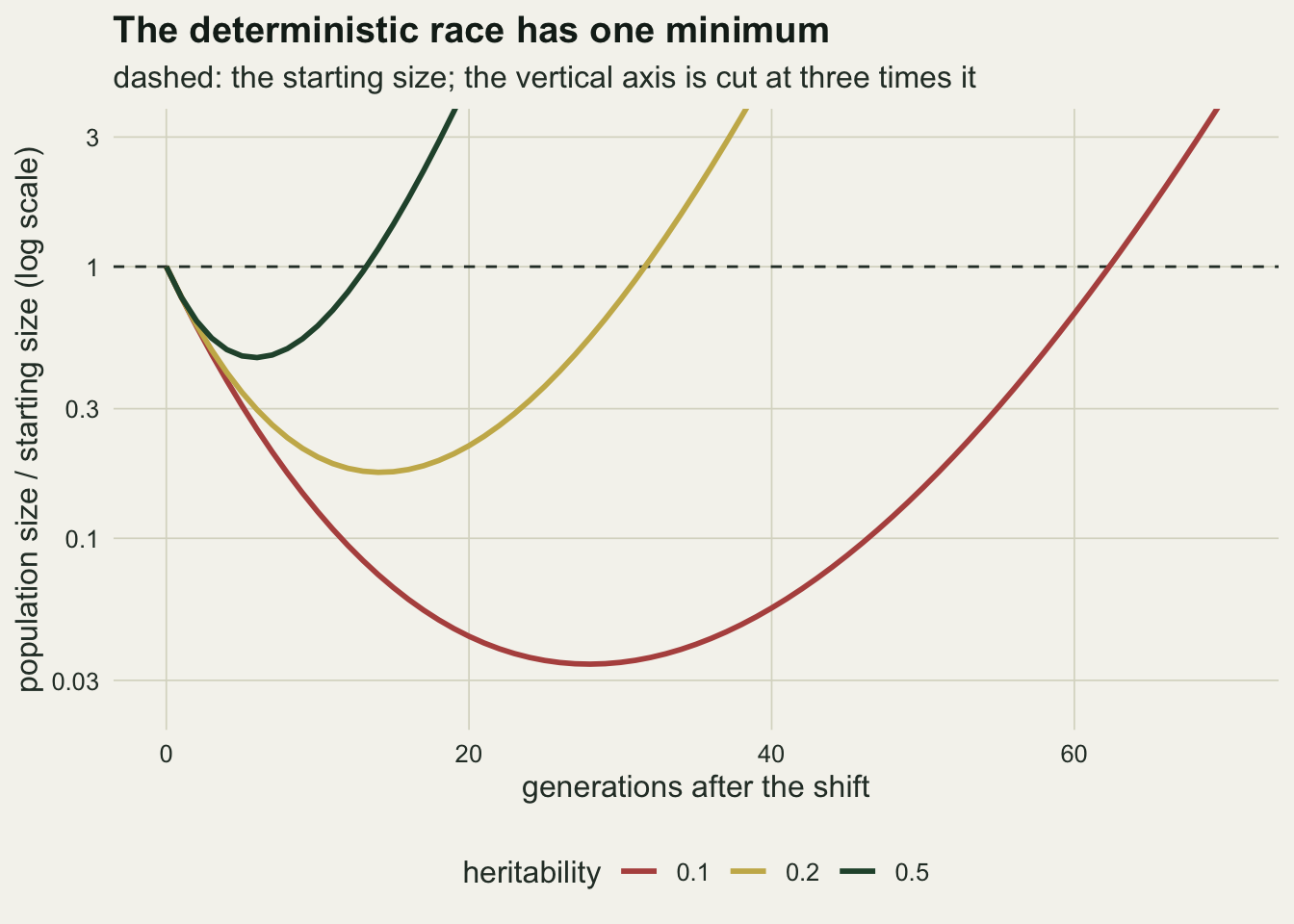
An individual-based version with the same parameters
The simulated population is sexual and follows the infinitesimal model. Each individual has a breeding value and a phenotype equal to that value plus a fresh environmental deviation with variance E. Its fitness is the same Gaussian function as above. The number of offspring in the next generation is a Poisson draw with mean equal to the summed fitness of the population, which is the same as every individual having a Poisson number of offspring with mean equal to its own fitness. Each offspring gets two parents drawn from the population with probability proportional to fitness (selfing is not excluded, and happens with probability of order one over N), and its breeding value is the midparent value plus a segregation deviation with variance G/2, where G is the starting additive variance. That variance is held fixed, so inbreeding does not erode it; selection does, and that is measured below.
Two ecological assumptions are added that the deterministic model does not have. The population is capped at its starting size, as if it were sitting at carrying capacity when the environment changed. And a population counts as rescued if it is alive after 150 generations. To keep the knit short, a replicate is taken out of the simulation early, and counted as rescued, once it is back at its starting size and the mean fitness implied by its mean breeding value is at least one; that shortcut is checked against the full run further down.
All replicates of a cell run in one vector, sorted by replicate, so each generation is a handful of vector operations whatever the number of replicates. Parents are drawn by placing uniform numbers inside each replicate’s stretch of the cumulative fitness vector and finding the interval.
sim_rescue <- function(n0, h2, shift, n_rep, horizon = t_max,
                       stop_safe = TRUE, track = FALSE) {
  g_var <- h2 * p_var
  e_var <- p_var - g_var
  rep_n <- rep.int(n0, n_rep)
  safe  <- logical(n_rep)
  n_low <- rep.int(n0, n_rep)
  t_low <- integer(n_rep)
  n_mat <- if (track) matrix(0L, n_rep, horizon) else NULL
  d_bar <- g_bar <- rep(NA_real_, horizon)
  a_val <- rnorm(n0 * n_rep, 0, sqrt(g_var))
  for (tt in seq_len(horizon)) {
    if (sum(rep_n) == 0) break
    z_val <- a_val + rnorm(length(a_val), 0, sqrt(e_var))
    w_val <- w_max * exp(-(z_val - shift)^2 / (2 * omega2))
    cum_w <- c(0, cumsum(w_val))
    ends  <- cumsum(rep_n)
    base  <- cum_w[ends - rep_n + 1]
    tot   <- cum_w[ends + 1] - base
    n_new <- pmin(rpois(n_rep, tot), n0)
    dips  <- n_new < n_low & !safe
    n_low[dips] <- n_new[dips]
    t_low[dips] <- tt
    rep_n <- n_new
    if (track) n_mat[, tt] <- n_new
    n_off <- sum(n_new)
    if (n_off == 0) break
    grp   <- rep.int(seq_len(n_rep), n_new)
    i_one <- findInterval(base[grp] + runif(n_off) * tot[grp], cum_w)
    i_two <- findInterval(base[grp] + runif(n_off) * tot[grp], cum_w)
    a_val <- (a_val[i_one] + a_val[i_two]) / 2 +
      rnorm(n_off, 0, sqrt(g_var / 2))
    live    <- which(n_new > 0)
    bv_mean <- rowsum(a_val, grp, reorder = TRUE)[, 1] / n_new[live]
    if (track) {
      bv_sq    <- rowsum(a_val^2, grp, reorder = TRUE)[, 1] / n_new[live]
      d_bar[tt] <- mean(shift - bv_mean)
      g_bar[tt] <- mean(bv_sq - bv_mean^2)
    }
    if (stop_safe) {
      now_safe <- live[n_new[live] == n0 & wbar_fun(shift - bv_mean) >= 1]
      if (length(now_safe) > 0) {
        safe[now_safe]  <- TRUE
        a_val           <- a_val[!(grp %in% now_safe)]
        rep_n[now_safe] <- 0L
      }
    }
  }
  list(rescued = safe | rep_n > 0, t_low = t_low, n_mat = n_mat,
       d_bar = d_bar, g_bar = g_bar)
}
Where the individual-based model and the deterministic one should agree is a large population over the first generations, before anything goes extinct. The check below runs populations of two thousand at the highest heritability for twenty generations and compares the mean distance to the optimum with the deterministic path. It also records the additive variance, because selection on the phenotype removes some of it every generation (the Bulmer effect, which the breeder’s equation post shows under truncation selection), and the deterministic model assumes it does not.
n_big   <- 2000
rep_big <- 20
gen_chk <- 20
h2_chk  <- 0.5
set.seed(5520)
big_run <- sim_rescue(n_big, h2_chk, shift_use, rep_big, horizon = gen_chk,
                      stop_safe = FALSE, track = TRUE)
gh_chk  <- gh_path(h2_chk, shift_use, gen_chk)
d_sim5  <- big_run$d_bar[5]
d_gh5   <- gh_chk$d[6]
d_sim20 <- big_run$d_bar[gen_chk]
d_gh20  <- gh_chk$d[gen_chk + 1]

g_start <- h2_chk * p_var
g_mean  <- mean(big_run$g_bar)
g_eq <- g_start
for (i in 1:200) {
  g_sel <- g_eq - g_eq^2 / (omega2 + g_eq + p_var - g_start)
  g_eq  <- g_sel / 2 + g_start / 2
}
g_drop <- 100 * (1 - g_mean / g_start)
d_geq20 <- shift_use * (1 - g_eq * gamma_s)^gen_chk
After five generations the simulated mean distance to the optimum is 2.732 against a deterministic 2.708. After twenty it is 1.316 against 1.255: the simulated population is a little behind, and the additive variance accounts for the lag. It averages 0.477 over the twenty generations instead of 0.50, 4.7 per cent less, and the infinitesimal recursion for Gaussian selection (selected variance G minus G squared over omega squared plus P, then half of it plus half of the segregation variance) settles at 0.477. Running the deterministic path with that equilibrium variance instead of the starting one gives a distance of 1.316 at generation twenty, against the simulated 1.316. So heritability is not held exactly constant: it falls quickly to a slightly lower equilibrium and stays there, and the deterministic reference, which uses the starting G, adapts a little faster than the simulation. Because the selection is weak, the difference is small; the loss per generation scales with G squared over omega squared plus P, so it grows as the fitness function narrows.
Rescue probability against starting size
The grid is fixed at six starting sizes from 25 to 800 and the three heritabilities, with 400 replicates per cell. That replication puts the Monte Carlo standard error of any rescue probability at 0.025 or below.
n0_grid <- c(25, 50, 100, 200, 400, 800)
n_rep   <- 400
mc_se_max <- sqrt(0.25 / n_rep)

run_cell <- function(n0, h2, shift) {
  s_out <- sim_rescue(n0, h2, shift, n_rep)
  p_hat <- mean(s_out$rescued)
  c(n0 = n0, h2 = h2, shift = shift, p = p_hat,
    se = sqrt(p_hat * (1 - p_hat) / n_rep),
    t_low = if (any(s_out$rescued)) median(s_out$t_low[s_out$rescued]) else NA)
}

set.seed(7731)
cells_main <- expand.grid(n0 = n0_grid, h2 = h2_grid)
res_main <- as.data.frame(t(mapply(run_cell, cells_main$n0, cells_main$h2,
                                   MoreArgs = list(shift = shift_use))))
res_main$gh_min <- res_main$n0 * gh_tab$min_rel[match(res_main$h2, gh_tab$h2)]
res_main$gh_says <- res_main$gh_min >= n_crit

p_at <- function(n0, h2) res_main$p[res_main$n0 == n0 & res_main$h2 == h2]
gh_yes <- res_main[res_main$gh_says, ]
n_gh_yes    <- nrow(gh_yes)
n_gh_yes_lt <- sum(gh_yes$p < 0.5)
worst_yes   <- gh_yes[which.min(gh_yes$p), ]
gh_no  <- res_main[!res_main$gh_says, ]
n_gh_no <- nrow(gh_no)
best_no <- gh_no[which.max(gh_no$p), ]

tl_h2 <- function(h2) median(res_main$t_low[res_main$h2 == h2 & res_main$n0 >= 100])
The deterministic verdict leaves out two kinds of chance at once, and the individual-based model has both. One is demographic: even with mean fitness following the deterministic path exactly, each individual leaves a Poisson number of offspring, and a small population can die out by bad luck in its births. The other is genetic: in a small population the mean breeding value itself wanders, because the founders are a sample and each generation’s parents are a sample of the last. The first can be computed exactly. Give every individual a Poisson number of offspring with mean equal to the deterministic mean fitness of its generation, and the population is a branching process whose extinction probability by the horizon comes from composing the offspring generating functions, one per generation. It keeps the deterministic mean path and adds demographic noise only, with every member of a generation sharing the same mean fitness. Whatever separates it from the individual-based model is therefore the drift of the mean together with three things the branching process also leaves out: fitness differences between individuals of the same generation (which make offspring numbers more variable than a Poisson count), the Bulmer loss of variance measured above, and the ceiling, which the second function below checks.
m_path <- function(h2, shift) wbar_fun(shift * (1 - h2 * p_var * gamma_s)^(0:(t_max - 1)))
bp_rescue <- function(h2, shift, n0) {
  m <- m_path(h2, shift)
  s <- 0
  for (tt in t_max:1) s <- exp(m[tt] * (s - 1))
  1 - s^n0
}
dem_cap <- function(h2, shift, n0, n_sim = 4000) {
  m <- m_path(h2, shift)
  n <- rep.int(n0, n_sim)
  for (tt in seq_len(t_max)) n <- pmin(rpois(n_sim, n * m[tt]), n0)
  mean(n > 0)
}
res_main$bp <- mapply(bp_rescue, res_main$h2, shift_use, res_main$n0)
res_main$gap <- res_main$bp - res_main$p
worst_gap <- res_main[which.max(res_main$gap), ]
n_gap_sig <- sum(res_main$gap > 2 * res_main$se & res_main$se > 0)
bp_at <- function(n0, h2) res_main$bp[res_main$n0 == n0 & res_main$h2 == h2]
bp_n0_half <- function(h2, shift) log(0.5) / log(1 - bp_rescue(h2, shift, 1))

set.seed(2718)
cap_p <- mapply(dem_cap, res_main$h2, shift_use, res_main$n0)
cap_gap <- max(abs(cap_p - res_main$bp))
The branching process sits above the individual-based model in most of the grid; the simulation is slightly above it only in two cells at a heritability of 0.1, where rescue is rare. At a starting size of 100 and a heritability of 0.2 it rescues 0.807 of populations against the simulated 0.645, and at 25 with 0.5 it rescues 0.835 against 0.645. The largest gap in this grid is 0.190 (starting size 25, heritability 0.5), and in 11 of the 18 cells the simulated probability is more than two Monte Carlo standard errors below the branching process. The ceiling does not explain it: the same demographic model with the population capped at its starting size, simulated 4000 times per cell, differs from the uncapped branching process by at most 0.010. Demographic chance alone already asks for a much larger starting population than the deterministic threshold: even odds need 42 founders at a heritability of 0.2, where the deterministic model rescues anything above 5.7. The drifting mean of a small population, and the other ingredients the branching process lacks, then take a further bite.
At a heritability of 0.2 the rescue probability climbs from 0.263 at a starting size of 25 to 0.645 at 100 and 1.000 at 800. At 0.5 it is already 0.645 at 25 and 0.970 at 100. At 0.1 it goes from 0.083 to 0.665 over the whole grid. Starting size and heritability both matter, and they trade against each other: in these cells a population of 25 with a heritability of 0.5 is about as safe as one of 100 with 0.2, whose rescue probability is 0.645.
Against the deterministic verdict with a threshold of one individual, 17 of the 18 cells are predicted to be rescued. In 6 of those the simulated rescue probability is below one half, and the worst is a starting size of 50 at a heritability of 0.1, rescued in 0.098 of runs, where the deterministic minimum is 1.72 individuals. The error does not run only one way. The one cell the deterministic model calls extinct is rescued in 0.083 of runs (starting size 25, heritability 0.1): a deterministic minimum below one individual is not certain death for a population that can get lucky, both in the order of its births and in which of its members happen to breed.
The timing of the trough, by contrast, is where the deterministic model puts it. Among rescued populations, the median over starting sizes of 100 or more of each cell’s median generation of the smallest census is 14.5 at a heritability of 0.2 against a deterministic 14, and 6.0 at 0.5 against 6. What the deterministic model gets wrong is not when the population is smallest but what being that small costs.
res_plot <- res_main
res_plot$h2 <- sprintf("%.1f", res_plot$h2)
star_df <- data.frame(n0_star = gh_tab$n0_star, h2 = sprintf("%.1f", gh_tab$h2))
n0_line <- exp(seq(log(2), log(800), length.out = 120))
bp_line <- do.call(rbind, lapply(h2_grid, function(h)
  data.frame(n0 = n0_line, p = bp_rescue(h, shift_use, n0_line), h2 = sprintf("%.1f", h))))
ggplot(res_plot, aes(n0, p, colour = h2)) +
  geom_vline(data = star_df, aes(xintercept = n0_star, colour = h2),
             linetype = "dashed", linewidth = 0.6) +
  geom_line(data = bp_line, linewidth = 0.5, alpha = 0.8) +
  geom_line(linewidth = 0.9) +
  geom_errorbar(aes(ymin = pmax(p - 1.96 * se, 0), ymax = pmin(p + 1.96 * se, 1)),
                width = 0.05, linewidth = 0.5) +
  geom_point(size = 2.2) +
  scale_x_log10(breaks = c(2, 5, 10, 25, 50, 100, 200, 400, 800)) +
  scale_y_continuous(limits = c(0, 1)) +
  scale_colour_manual(values = h2_cols, name = "heritability") +
  labs(x = "starting population size (log scale)", y = "probability of rescue",
       title = "Deterministic rescue is not stochastic rescue",
       subtitle = "thick: individual-based; thin: branching process; dashed: minimum of one") +
  theme_datasheet() +
  theme(legend.position = "bottom")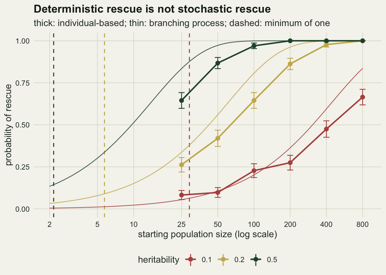
What a single cell looks like
The probabilities hide how different the rescued and the lost populations are. The run below keeps every census for a starting size of 100 at a heritability of 0.2, without the early exit, so the rescued populations are followed to the horizon.
n0_traj <- 100
h2_traj <- 0.2
rep_traj <- 200
set.seed(9187)
traj_run <- sim_rescue(n0_traj, h2_traj, shift_use, rep_traj, horizon = 60,
                       stop_safe = FALSE, track = TRUE)
alive_60 <- traj_run$n_mat[, 60] > 0
p_traj   <- mean(alive_60)
ext_gen  <- apply(traj_run$n_mat[!alive_60, , drop = FALSE], 1,
                  function(v) which(v == 0)[1])
ext_med  <- median(ext_gen)
low_resc <- apply(traj_run$n_mat[alive_60, , drop = FALSE], 1, min)
low_med  <- median(low_resc)
gh_low_traj <- n0_traj * gh_tab$min_rel[gh_tab$h2 == h2_traj]
By generation 60, 0.610 of the 200 populations are alive. The lost ones have a median generation of extinction of 18, after the deterministic minimum at generation 14: many populations were still dying while the deterministic trajectory was already climbing, because a population that has drifted to a handful of individuals needs several generations of positive growth to get out of range of a run of bad draws. The survivors went through a median smallest census of 15 individuals, against a deterministic minimum of 17.5. Surviving did not require avoiding the trough; at least half the survivors fell below the deterministic minimum and came back.
traj_long <- data.frame(
  gen = rep(seq_len(60), each = rep_traj),
  n = as.vector(traj_run$n_mat),
  run = rep(seq_len(rep_traj), times = 60),
  fate = rep(ifelse(alive_60, "alive at 60", "extinct"), times = 60))
traj_long <- traj_long[traj_long$n > 0, ]
gh_traj <- gh_path(h2_traj, shift_use, 60)
gh_traj$n <- pmin(n0_traj * gh_traj$n_rel, n0_traj)
ggplot(traj_long, aes(gen, n, group = run, colour = fate)) +
  geom_line(linewidth = 0.3, alpha = 0.45) +
  geom_line(data = gh_traj, aes(gen, n), inherit.aes = FALSE,
            colour = te_ink, linewidth = 1.1) +
  scale_colour_manual(values = c("alive at 60" = te_forest, "extinct" = te_rust),
                      name = NULL) +
  labs(x = "generation", y = "population size",
       title = "The trough decides it",
       subtitle = "black: deterministic trajectory, capped at the starting size") +
  guides(colour = guide_legend(override.aes = list(linewidth = 1.2, alpha = 1))) +
  theme_datasheet() +
  theme(legend.position = "bottom")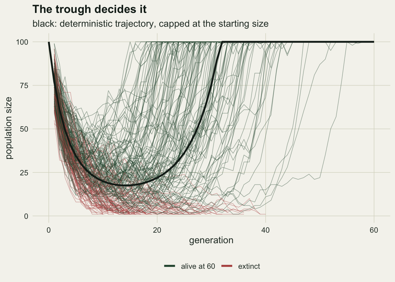
Three shift sizes, one predictor
The shift was fixed at 3.5 so far, and the numbers above belong to that value. Repeating the grid at shifts of 3 and 4 tests whether anything carries over. The quantity that might carry over is the deterministic minimum itself, in individuals: if extinction is mostly a matter of how few individuals are left at the bottom, then rescue probability should line up on the deterministic minimum whatever combination of shift, heritability and starting size produced it.
shift_grid <- c(3, 4)
cells_more <- expand.grid(n0 = n0_grid, h2 = h2_grid, shift = shift_grid)
set.seed(3306)
res_more <- as.data.frame(t(mapply(run_cell, cells_more$n0, cells_more$h2,
                                   cells_more$shift)))
res_all <- rbind(res_main[, names(res_more)], res_more)

gh_all <- as.data.frame(t(mapply(gh_summary, res_all$h2, res_all$shift)))
res_all$gh_min <- res_all$n0 * gh_all$min_rel
res_all$t_back <- gh_all$t_back
back_max <- max(res_all$t_back, na.rm = TRUE)
back_na  <- sum(is.na(res_all$t_back))

half_point <- function(cell_rows) {
  cell_rows <- cell_rows[order(cell_rows$gh_min), ]
  i_up <- which(cell_rows$p >= 0.5)[1]
  if (is.na(i_up) || i_up == 1) return(NA)
  x_lo <- log(cell_rows$gh_min[i_up - 1]); x_hi <- log(cell_rows$gh_min[i_up])
  y_lo <- cell_rows$p[i_up - 1]; y_hi <- cell_rows$p[i_up]
  exp(x_lo + (0.5 - y_lo) * (x_hi - x_lo) / (y_hi - y_lo))
}
half_tab <- expand.grid(h2 = h2_grid, shift = c(3, shift_use, 4))
half_tab$n_half <- mapply(function(h, s) half_point(res_all[res_all$h2 == h & res_all$shift == s, ]),
                          half_tab$h2, half_tab$shift)
half_ok  <- half_tab[!is.na(half_tab$n_half), ]
half_lo  <- min(half_ok$n_half)
half_hi  <- max(half_ok$n_half)
half_n   <- nrow(half_ok)
half_ok$min_rel <- mapply(function(h, s) gh_summary(h, s)[["min_rel"]],
                          half_ok$h2, half_ok$shift)
half_ok$n0_half <- half_ok$n_half / half_ok$min_rel
n0_half_lo <- min(half_ok$n0_half)
n0_half_hi <- max(half_ok$n0_half)
hv <- function(h, s) half_ok$n_half[half_ok$h2 == h & half_ok$shift == s]

p_s <- function(n0, h2, shift) res_all$p[res_all$n0 == n0 & res_all$h2 == h2 & res_all$shift == shift]

half_ok$bp_half <- mapply(function(h, s) bp_n0_half(h, s), half_ok$h2, half_ok$shift) * half_ok$min_rel
bp_half_lo <- min(half_ok$bp_half)
bp_half_hi <- max(half_ok$bp_half)
half_ratio <- half_ok$n_half / half_ok$bp_half
bpv <- function(h, s) half_ok$bp_half[half_ok$h2 == h & half_ok$shift == s]

set.seed(1618)
n_boot <- 1000
boot_half <- replicate(n_boot, {
  r_b <- res_all
  r_b$p <- rbinom(nrow(r_b), n_rep, r_b$p) / n_rep
  mapply(function(h, s) half_point(r_b[r_b$h2 == h & r_b$shift == s, ]), half_ok$h2, half_ok$shift)
})
half_ok$ci_lo <- apply(boot_half, 1, quantile, 0.025, na.rm = TRUE)
half_ok$ci_hi <- apply(boot_half, 1, quantile, 0.975, na.rm = TRUE)
ord_share <- mean(apply(boot_half, 2, function(v)
  min(v[half_ok$h2 == 0.1]) > max(v[half_ok$h2 == 0.5])), na.rm = TRUE)
hci <- function(h, s) {
  i <- which(half_ok$h2 == h & half_ok$shift == s)
  sprintf("%.1f [%.1f, %.1f]", half_ok$n_half[i], half_ok$ci_lo[i], half_ok$ci_hi[i])
}
half_ok$logit_half <- mapply(function(h, s) {
  r_c <- res_all[res_all$h2 == h & res_all$shift == s, ]
  f_c <- suppressWarnings(glm(cbind(p * n_rep, (1 - p) * n_rep) ~ log(gh_min),
                              family = binomial, data = r_c))
  exp(-coef(f_c)[1] / coef(f_c)[2])
}, half_ok$h2, half_ok$shift)
logit_diff <- max(abs(half_ok$logit_half - half_ok$n_half))
The deterministic recovery time is at most 99 generations over the 54 cells, every one of which recovers, inside the horizon of 150, so a population alive at the horizon is not one that is still sliding.
The shift changes everything on the starting size axis. At a heritability of 0.2 and a starting size of 50, the rescue probability is 0.912 after a shift of 3, 0.420 after 3.5 and 0.087 after 4. Going from 3 to 3.5 costs more than doubling the population to 100 gives back, since that doubling at a shift of 3.5 raises the probability only to 0.645.
On the deterministic minimum axis the cells come much closer together. For each combination of shift and heritability whose rescue probability crosses one half inside the grid (5 of the nine), interpolating on the log of the deterministic minimum gives the minimum at which half the populations are rescued. It lies between 8.4 and 15.1 individuals. A parametric bootstrap, redrawing every cell as a binomial with 400 trials and repeating the interpolation 1000 times, gives the intervals quoted below in square brackets; a logistic regression of rescue on the log of the minimum, fitted per combination instead of the interpolation, moves no half point by more than 1.0 individuals. The starting sizes that produce those minima run from 28 to 763, so the deterministic minimum removes most of the spread that the shift puts on the starting size axis.
What is left is ordered by heritability, and it is consistent across shifts. At a heritability of 0.1 the half point is 15.1 [13.8, 17.0] individuals after a shift of 3 and 15.1 [12.9, 17.3] after 3.5; at 0.2 it is 11.2 [9.9, 12.5] after 3.5 and 12.1 [10.1, 12.7] after 4; at 0.5 it is 8.4 [7.3, 9.5] after 4, the only shift at which that half point falls inside the grid. Every half point at 0.1 exceeds the one at 0.5 in 100 per cent of bootstrap draws; the two at 0.2 are not distinguishable from each other.
The branching process splits that number in two. With demographic chance alone, on the same deterministic mean path, even odds arrive at a deterministic minimum of 9.3 and 10.6 individuals at a heritability of 0.1, 7.4 and 7.6 at 0.2, and 4.8 at 0.5. Those values need no simulation; they come from the extinction probability of a single founder. So demographic chance already moves the threshold from one individual to between 4.8 and 10.6, and the heritability ordering is already there: a lower heritability gives a longer, flatter trough, the population spends more generations near its minimum, and each of those generations is another chance for a run of bad births. The individual-based model then asks for 1.4 to 1.7 times as many individuals as the branching process in the same combination. That extra factor is everything the branching process leaves out, and it is not a pure measure of drift. The drift part works like this: a small population’s mean breeding value drifts in both directions around the deterministic path, and the populations pushed behind it sit in a deeper, longer trough, which costs more than the ones pushed ahead gain. Two other omissions push the same way: individuals of one generation differ in fitness, so offspring numbers vary more than a Poisson count with the mean fitness would, and the Bulmer effect slows adaptation slightly. None of the five half points, in either model, is anywhere near one individual, the threshold that makes the deterministic verdict literal.
res_all_plot <- res_all
res_all_plot$h2    <- sprintf("%.1f", res_all_plot$h2)
res_all_plot$shift <- sprintf("shift %.1f", res_all_plot$shift)
combo <- expand.grid(h2 = h2_grid, shift = c(3, shift_use, 4))
bp_curves <- do.call(rbind, lapply(seq_len(nrow(combo)), function(i) {
  m_rel <- gh_summary(combo$h2[i], combo$shift[i])[["min_rel"]]
  n0_c  <- exp(seq(log(25), log(800), length.out = 80))
  data.frame(gh_min = n0_c * m_rel, p = bp_rescue(combo$h2[i], combo$shift[i], n0_c),
             h2 = sprintf("%.1f", combo$h2[i]), combo = i)
}))
ggplot(res_all_plot, aes(gh_min, p, colour = h2, shape = shift)) +
  geom_vline(xintercept = n_crit, linetype = "dashed", colour = te_body, linewidth = 0.5) +
  geom_hline(yintercept = 0.5, linetype = "dotted", colour = te_body, linewidth = 0.5) +
  geom_line(data = bp_curves, aes(gh_min, p, colour = h2, group = combo),
            inherit.aes = FALSE, linewidth = 0.4, alpha = 0.7) +
  geom_point(size = 2.4, stroke = 0.9) +
  scale_x_log10(breaks = c(0.01, 0.1, 1, 10, 100),
                labels = c("0.01", "0.1", "1", "10", "100")) +
  scale_shape_manual(values = c(1, 16, 2), name = NULL) +
  scale_colour_manual(values = h2_cols, name = "heritability") +
  labs(x = "deterministic minimum population size (log scale)",
       y = "probability of rescue",
       title = "The deterministic minimum lines the cells up",
       subtitle = "lines: branching process; dashed: one individual; dotted: one half") +
  theme_datasheet() +
  theme(legend.position = "bottom", legend.box = "vertical")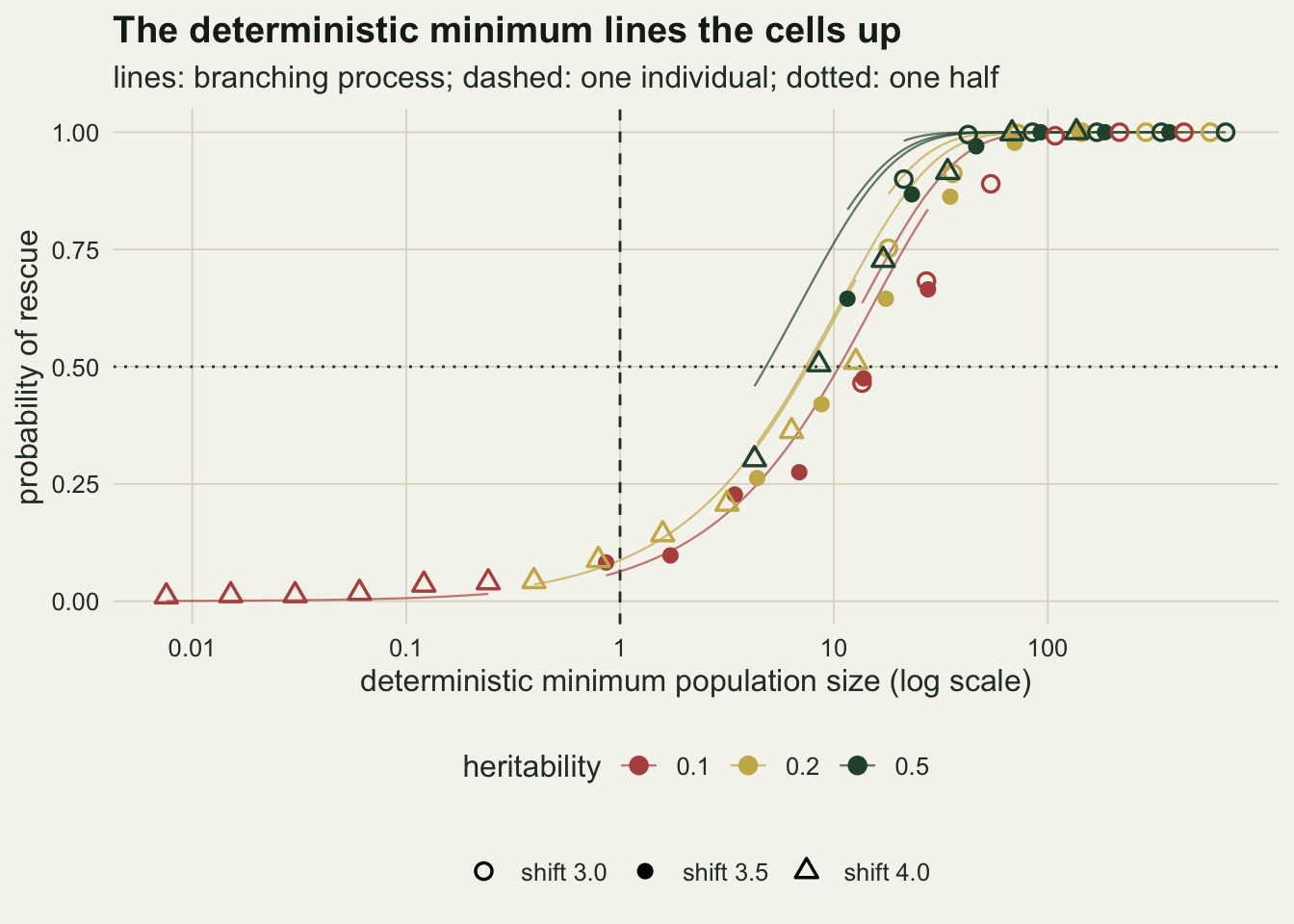
Checking the early exit
The early exit counts a replicate as rescued once it is back at its starting size with mean fitness at or above one. The check below reruns three small cells, where a population at its ceiling is most at risk, with the exit switched off and the full horizon simulated.
n_chk_rep <- 2000
chk_cells <- data.frame(n0 = c(25, 25, 25), h2 = c(0.2, 0.5, 0.1),
                        shift = c(3.5, 3, 3.5))
set.seed(6620)
chk_out <- t(sapply(seq_len(nrow(chk_cells)), function(i) {
  p_fast <- mean(sim_rescue(chk_cells$n0[i], chk_cells$h2[i], chk_cells$shift[i],
                            n_chk_rep)$rescued)
  p_full <- mean(sim_rescue(chk_cells$n0[i], chk_cells$h2[i], chk_cells$shift[i],
                            n_chk_rep, stop_safe = FALSE)$rescued)
  se_diff <- sqrt((p_fast * (1 - p_fast) + p_full * (1 - p_full)) / n_chk_rep)
  c(p_fast = p_fast, p_full = p_full, z = (p_fast - p_full) / se_diff)
}))
z_max <- max(abs(chk_out[, "z"]))
d_max <- max(abs(chk_out[, "p_fast"] - chk_out[, "p_full"]))

n0_small <- 10
p_fast10 <- mean(sim_rescue(n0_small, 0.5, 3, n_chk_rep)$rescued)
p_full10 <- mean(sim_rescue(n0_small, 0.5, 3, n_chk_rep, stop_safe = FALSE)$rescued)
With 2000 replicates each, the largest difference between the shortcut and the full run is 0.009, or 0.9 standard errors of the difference. At a starting size of 25 the shortcut is not changing the answer. At a starting size of 10 (heritability 0.5, shift 3) it does: the shortcut says 0.663 and the full run 0.461, because a population held at a ceiling of ten still dies often enough after adapting to matter. That is why the grid starts at 25.
What to report
Report the shift in units of phenotypic standard deviation together with the width of the fitness function, or report the starting mean fitness they imply. In this post a change of half a standard deviation in the shift moved the rescue probability at a fixed starting size from 0.912 to 0.420, so a rescue probability quoted without the shift carries almost no information.
Report the deterministic minimum population size in individuals, not only whether the minimum clears a threshold. It is one line of R from the shift, the heritability, the width of selection and the starting size, and in these simulations it ordered the rescue probability across shifts far better than starting size did. If a threshold is needed, one individual is the wrong one: the populations here reached even odds of rescue only when the deterministic minimum was between 8 and 15 individuals, and the lower the heritability, the higher that figure. The branching process on the deterministic mean path, a few lines of R with no simulation, gives the demographic part of that threshold (5 to 11 here) and is a better quick reference than the threshold of one; it is still optimistic, because it ignores drift in the mean and the spread of fitness among individuals.
Say whether additive variance was held fixed, and if it was not, what happened to it. In the infinitesimal model with Gaussian selection it drops by 4.7 per cent in a few generations at the width used here, and the deterministic path with the reduced variance matched the simulation where the path with the starting variance did not.
Give the definition of rescue and the horizon. Alive after a fixed number of generations, back to the starting size, and eventual persistence in a model with no ceiling are three different quantities, and they separate most for very small populations, where the shortcut used here stopped being harmless at a ceiling of ten.
Honest limits
The environment changes once and then stays put. Many real changes are gradual, and a steadily moving optimum produces a lag that the population carries indefinitely rather than a single trough; Lande and Shannon treat that case, and its critical rate of change is a different quantity from anything measured here. The abrupt shift was chosen because it is the case with a closed form deterministic path to compare against.
Inheritance is infinitesimal with a fixed segregation variance, which means drift and inbreeding can erode only the half of the additive variance carried between families, never the segregation half, however small the population gets. A population that spends ten generations at a dozen individuals would lose a noticeable part of its variance at a finite number of loci, and would adapt more slowly than the simulation lets it. The rescue probabilities at small starting sizes are therefore on the generous side, and more so at low heritability, where the trough is long.
Genetic variance is standing variation only. No new mutations arise, and a population that has used up its variation cannot find more. Bell and Gonzalez’s yeast experiments, and much of the rescue literature that Carlson and colleagues review, turn on new mutations of large effect, and there population size enters a second time, because a larger population also samples more new mutations.
The fitness function has a single fixed width and a single maximum growth rate, and the demography is Poisson with a hard ceiling. Environmental stochasticity, which adds correlated bad years on top of the demographic noise, is absent; so is any density dependence below the ceiling, and so are sexes, age structure and Allee effects. Most of these would be expected to lower the rescue probability for a given deterministic minimum, and none of the half points above should be carried to a species with any of them without rerunning the code.
The grid is coarse. Three shifts and three heritabilities give nine combinations, each with six starting sizes, and only five of them cross one half inside the grid, so each half point rests on a linear interpolation between two cells, each with a Monte Carlo standard error of up to 0.025. The bootstrap intervals above carry that uncertainty, but not the choice of interpolation. The split between demographic and genetic chance is also a difference of two models rather than a separate measurement: the part assigned to drift in the mean also carries founder sampling and selfing, the spread of fitness among individuals within a generation, the Bulmer loss of variance, and the small effect of the ceiling measured above.
References
Gomulkiewicz R, Holt RD 1995 Evolution 49(1):201-207 (10.1111/j.1558-5646.1995.tb05971.x)
Lande R 1976 Evolution 30(2):314-334 (10.1111/j.1558-5646.1976.tb00911.x)
Lande R, Shannon S 1996 Evolution 50(1):434-437 (10.1111/j.1558-5646.1996.tb04504.x)
Bell G, Gonzalez A 2009 Ecology Letters 12(9):942-948 (10.1111/j.1461-0248.2009.01350.x)
Carlson SM, Cunningham CJ, Westley PAH 2014 Trends in Ecology and Evolution 29(9):521-530 (10.1016/j.tree.2014.06.005)