The breeder’s equation in R

Predict the response to selection in R with the breeder’s equation R = h squared S, estimate realised heritability, and see why it drifts over generations.

The selection differential tells you how hard selection pushed a trait within one generation. It says nothing about whether the population actually moves. A trait can be under fierce selection and go nowhere if none of its variation is inherited. The bridge from selection to evolution is the breeder’s equation, and its whole content is one line:

\[ R = h^2 S. \]

The response to selection R, the change in trait mean from one generation to the next, equals the narrow-sense heritability h^2 (the fraction of phenotypic variance that is additive genetic) times the selection differential S. This post builds a population where we know h^2 exactly, applies selection, and checks that the equation predicts what happens. Then it shows where the rule quietly stops working.

A population with a known heritability

Each individual gets an additive breeding value a and an independent environmental deviation. The phenotype is their sum. Heritability is the additive variance divided by the total.

set.seed(432)
VA <- 4; VE <- 6; mu <- 50
h2_true <- VA / (VA + VE)
n <- 5000; p_sel <- 0.20

make_pop <- function(a) data.frame(a = a, z = mu + a + rnorm(length(a), 0, sqrt(VE)))
breed <- function(sel, n_off) {
  s <- sample(sel$a, n_off, TRUE); d <- sample(sel$a, n_off, TRUE)
  a_off <- (s + d) / 2 + rnorm(n_off, 0, sqrt(VA / 2))   # midparent + Mendelian sampling
  make_pop(a_off)
}
cat(sprintf("true heritability h2 = %.3f\n", h2_true))

true heritability h2 = 0.400

The breed function is the genetic engine: an offspring inherits the average breeding value of its two parents plus a Mendelian sampling term, which is the reshuffling of alleles that keeps variation alive even when parents are similar. The environment is redrawn fresh each generation, so it cannot be inherited.

One generation: the equation holds

Truncation selection keeps the top 20% by phenotype and breeds them at random.

pop <- make_pop(rnorm(n, 0, sqrt(VA)))
thr <- quantile(pop$z, 1 - p_sel)
sel <- pop[pop$z >= thr, ]
S   <- mean(sel$z) - mean(pop$z)
off <- breed(sel, n)
R   <- mean(off$z) - mean(pop$z)
cat(sprintf("S = %.3f   predicted R = h2*S = %.3f   observed R = %.3f\n",
            S, h2_true * S, R))

S = 4.346   predicted R = h2*S = 1.738   observed R = 1.771

The selection differential is 4.346 phenotype units: the breeders average that much above the population mean. The breeder’s equation predicts a response of 1.738, and the offspring generation actually shifts by 1.771. The prediction and the outcome agree to within sampling noise. Selection moved the mean by roughly 40% of the differential, exactly the heritability, because only 40% of the phenotypic spread was heritable and the rest stayed behind with the discarded environment.

Many generations: realised heritability

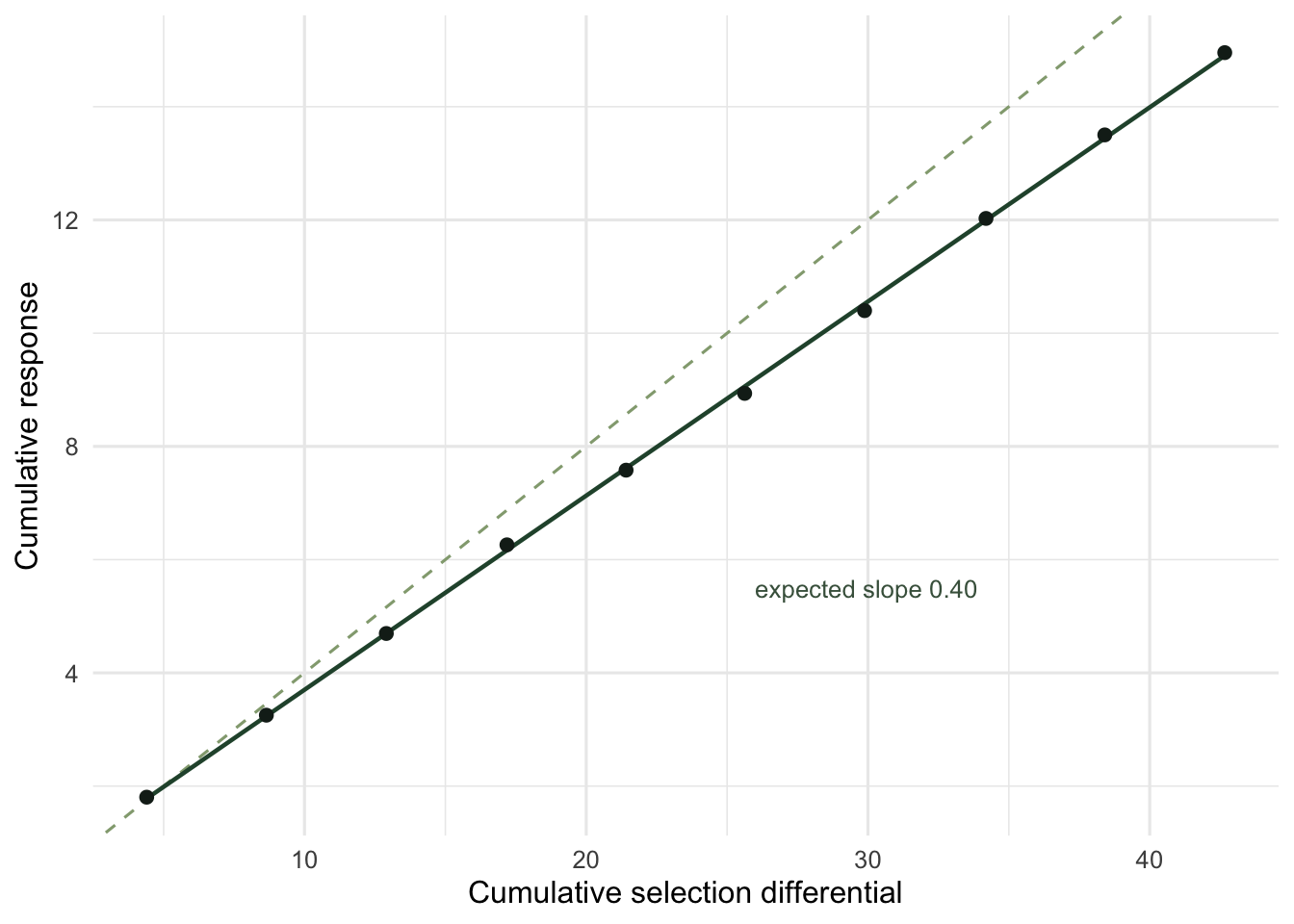
Run the same selection for ten generations and accumulate the differentials and responses. The slope of cumulative response on cumulative differential is the realised heritability, the estimate a breeder gets from a real selection experiment without ever measuring genes.

G <- 10
pop <- make_pop(rnorm(n, 0, sqrt(VA)))
base_mean <- mean(pop$z)
cumS <- 0; rows <- vector("list", G)
for (g in 1:G) {
  thr <- quantile(pop$z, 1 - p_sel); sel <- pop[pop$z >= thr, ]
  cumS <- cumS + (mean(sel$z) - mean(pop$z))
  pop  <- breed(sel, n)
  rows[[g]] <- data.frame(g = g, cumS = cumS, cumR = mean(pop$z) - base_mean)
}
df  <- do.call(rbind, rows)
fit <- lm(cumR ~ cumS, data = df)
cat(sprintf("realised h2 (slope) = %.3f   started from h2 = %.3f\n",
            coef(fit)[2], h2_true))

realised h2 (slope) = 0.343   started from h2 = 0.400

cat(sprintf("total response after %d generations = %.2f units (%.2f phenotypic SD)\n",
            G, tail(df$cumR, 1), tail(df$cumR, 1) / sqrt(VA + VE)))

total response after 10 generations = 14.95 units (4.73 phenotypic SD)

The realised heritability comes out at 0.343, below the 0.400 we built in. This is not a coding slip; it is the Bulmer effect. Sustained directional selection lines up the extremes and generates negative associations among the loci pulling the trait, which shrinks the additive variance to a new, lower equilibrium. The per-generation ratio of response to differential slides from 0.41 in the first generation toward 0.35 later on. The equation is exact for a single generation but the additive variance it depends on is not a constant, so a slope fitted across ten generations under-reports the starting heritability.

library(ggplot2)
ggplot(df, aes(cumS, cumR)) +
  geom_abline(slope = h2_true, intercept = 0, linetype = "dashed", colour = "#93a87f") +
  geom_smooth(method = "lm", se = FALSE, colour = "#275139", linewidth = 0.8) +
  geom_point(colour = "#16241d", size = 2) +
  annotate("text", x = 26, y = 5.5, label = "expected slope 0.40",
           colour = "#46604a", size = 3.4, hjust = 0) +
  labs(x = "Cumulative selection differential", y = "Cumulative response") +
  theme_minimal(base_size = 12)

`geom_smooth()` using formula = 'y ~ x'

Figure 1: Cumulative response against cumulative differential. The fitted realised heritability (green) falls below the line expected from the starting h squared of 0.4 (dashed), because sustained selection erodes the additive variance.

An honest limit: the stasis paradox

The deeper trouble appears in the wild. Many natural populations carry heritable traits under measurable directional selection, yet the trait mean sits still for decades. Plugging phenotypic S and a heritability into R = h^2 S predicts steady change that never comes; this is the stasis paradox (Merila and colleagues 2001).

The usual culprit is that the phenotypic differential is not what the equation actually needs. The genetic response is the covariance between breeding value and relative fitness (the Robertson-Price identity), and phenotypic S equals that only when the trait-fitness link is genetic. In observational field data, an individual in good condition is often both larger and more fecund because the environment made it so, not because size causes fitness. That environmentally induced covariance inflates S without any heritable basis, so the population does not respond (Morrissey and colleagues 2010). It is the same confounding that haunts any regression on observational data (see confounding and backdoor adjustment). The checking post returns to this as the central assumption a selection analysis rests on.

Related tutorials

• Selection differentials and gradients
• The multivariate breeder’s equation
• Checking a selection analysis
• Confounding and backdoor adjustment

References

Bulmer MG 1971. American Naturalist 105(943):201-211 (10.1086/282718)

Merila J, Sheldon BC, Kruuk LEB 2001. Genetica 112-113:199-222 (10.1023/A:1013391806317)

Morrissey MB, Kruuk LEB, Wilson AJ 2010. Journal of Evolutionary Biology 23(11):2277-2288 (10.1111/j.1420-9101.2010.02084.x)

Falconer DS, Mackay TFC 1996. Introduction to Quantitative Genetics, 4th ed. Longman. ISBN 978-0582243026