---
title: "Checking a selection analysis"
description: "Three diagnostics for selection gradients in R: collinearity among traits, non-normal fitness and the bootstrap, and reading the differential-gradient gap."
date: "2026-07-06 11:00"
categories: [evolutionary ecology, quantitative genetics, natural selection, model diagnostics, R, ecology tutorial]
image: thumbnail.png
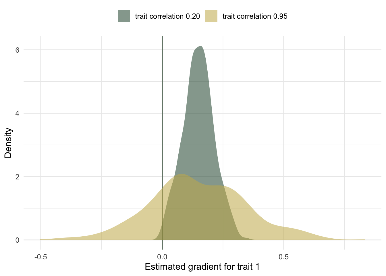
image-alt: "Two density curves of an estimated selection gradient under high and low trait collinearity, the high-collinearity curve much wider and spilling past zero"
---
A [selection gradient](../selection-differentials-and-gradients/) is a multiple regression of relative fitness on traits, so every failure mode of regression is also a failure mode of a selection analysis. Three of them bite hardest in field data: traits that are too correlated, fitness that is not remotely normal, and the quiet gap between what a trait experienced and what acted on it directly. This post works through all three in base R, then names the assumption no diagnostic can rescue.
## Check 1: collinearity among traits
Selection gradients isolate direct selection by holding the other traits constant. When two traits are nearly the same measurement, there is almost nothing left to hold constant, and the regression cannot tell them apart. Here are two traits correlated at 0.95, both under equal, genuine directional selection.
```{r}
#| label: collinear
set.seed(434)
n  <- 400
rx <- 0.95
x2 <- rnorm(n); x1 <- rx * x2 + sqrt(1 - rx^2) * rnorm(n)
W  <- rpois(n, exp(0.2 + 0.15 * x1 + 0.15 * x2)); w <- W / mean(W)
m  <- lm(w ~ x1 + x2)
vif <- 1 / (1 - summary(lm(x1 ~ x2))$r.squared)
cat(sprintf("VIF = %.1f\n", vif))
round(summary(m)$coefficients[c("x1", "x2"), ], 3)
```
The variance inflation factor is 9.0, so the standard errors are roughly three times what they would be for uncorrelated traits. The consequences are on display in this fit: the two gradients are 0.049 and 0.340 even though selection acted on them equally, one is "significant" and the other is not, and neither number means what it appears to. Run the same equal selection across many simulated datasets and the estimated gradient for trait 1 swings wildly.
```{r}
#| label: fig-instability
#| fig-cap: "The estimated selection gradient for one of two equally selected traits, across 400 simulated studies. Under high collinearity (0.95) the estimate is wide and spills past zero into the wrong sign; under low collinearity (0.2) it is tight and correct."
#| fig-alt: "Two overlaid density curves; the high-collinearity curve is broad and crosses zero, the low-collinearity curve is narrow and positive."
library(ggplot2)
te_canvas <- theme(plot.background  = element_rect(fill = "#f5f4ee", colour = NA),
                   panel.background = element_rect(fill = "#f5f4ee", colour = NA))
set.seed(707)
sim_beta1 <- function(rr, M = 400, nn = 200) {
  vapply(seq_len(M), function(k) {
    x2 <- rnorm(nn); x1 <- rr * x2 + sqrt(1 - rr^2) * rnorm(nn)
    W  <- rpois(nn, exp(0.2 + 0.15 * x1 + 0.15 * x2)); ww <- W / mean(W)
    coef(lm(ww ~ x1 + x2))[2]
  }, numeric(1))
}
b_hi <- sim_beta1(0.95); b_lo <- sim_beta1(0.2)
cat(sprintf("high-corr SD = %.3f, wrong sign in %.1f%% of studies; low-corr SD = %.3f\n",
            sd(b_hi), 100 * mean(b_hi < 0), sd(b_lo)))
dd <- rbind(data.frame(beta1 = b_hi, corr = "trait correlation 0.95"),
            data.frame(beta1 = b_lo, corr = "trait correlation 0.20"))
ggplot(dd, aes(beta1, fill = corr)) +
  geom_vline(xintercept = 0, colour = "#46604a", linewidth = 0.4) +
  geom_density(alpha = 0.55, colour = NA) +
  scale_fill_manual(values = c("trait correlation 0.95" = "#c9b458",
                               "trait correlation 0.20" = "#275139")) +
  labs(x = "Estimated gradient for trait 1", y = "Density", fill = NULL) +
  theme_minimal(base_size = 12) + te_canvas + theme(legend.position = "top")
```
Under the high correlation, 21.5% of studies would report the wrong sign for a trait that is truly under positive selection. The fix is not statistical: check the variance inflation factors before interpreting, and if two traits are effectively one, analyse a composite or drop one, rather than trusting a gradient the data cannot support.
## Check 2: fitness is not normal
Fitness is counts of offspring, or survived-or-not, never a tidy Gaussian. Lande and Arnold (1983) already answer the point estimate: the ordinary least squares gradient is the best linear approximation to the fitness surface whatever the fitness distribution, so the coefficient is still meaningful. The trap is the standard error. The `lm` standard error assumes constant-variance normal residuals, which count data violate, so the reported uncertainty is wrong even when the estimate is right. A bootstrap over individuals gives an honest interval.
```{r}
#| label: bootstrap
set.seed(505)
n2 <- 500
z  <- rnorm(n2)
W2 <- rpois(n2, exp(0.1 + 0.4 * z)); w2 <- W2 / mean(W2)
m2 <- lm(w2 ~ z)
B  <- 2000
bs <- vapply(seq_len(B), function(b) {
  i <- sample(n2, replace = TRUE); coef(lm(w2[i] ~ z[i]))[2]
}, numeric(1))
cat(sprintf("gradient = %.3f    lm SE = %.3f    bootstrap SE = %.3f\n",
            coef(m2)["z"], summary(m2)$coef["z", "Std. Error"], sd(bs)))
```
The gradient is 0.385 either way, but the model-based standard error, 0.040, understates the bootstrap value of 0.049. Report the estimate from the regression and the uncertainty from the resampling; a permutation test does the same job for the p-value (Mitchell-Olds and Shaw 1987).
## Check 3: read the differential-gradient gap
The gap between a trait's selection differential and its gradient is not a nuisance; it is a measurement. It equals the indirect selection the trait absorbed through its correlations, so a large gap flags a passenger. Take a trait `z1` that has no effect on fitness but correlates 0.7 with the real target `z2`.
```{r}
#| label: gap
set.seed(606)
nc <- 400
z2c <- rnorm(nc); z1c <- 0.7 * z2c + sqrt(1 - 0.7^2) * rnorm(nc)
Wc  <- rpois(nc, exp(0.2 + 0.35 * z2c)); wc <- Wc / mean(Wc)
S <- c(cov(z1c, wc), cov(z2c, wc))
b <- solve(cov(cbind(z1c, z2c))) %*% S
cat(sprintf("z1 (passenger): S = %.3f  beta = %.3f  gap = %.3f\n", S[1], b[1], S[1] - b[1]))
cat(sprintf("z2 (target) : S = %.3f beta = %.3f gap = %.3f\n", S[2], b[2], S[2] - b[2]))
```
The passenger `z1` has a healthy differential of 0.332 but a gradient of 0.060, a gap of 0.272: nearly all the selection it experienced was borrowed. The target `z2` has a small gap, 0.066: what it experienced is what acted on it. Always report both quantities, never just one; a differential without its gradient hides indirect selection, and a gradient without its differential hides how much total selection the trait actually saw.
## The assumption no check can save
All three diagnostics live inside the traits you measured. The one that can sink the whole analysis lives outside them. A selection gradient is phenotypic and descriptive: it attributes fitness to the measured traits, and if some unmeasured trait causes fitness and correlates with a measured one, its selection is misassigned to the trait you happened to record. This is omitted-variable bias wearing an evolutionary hat (see [confounding and backdoor adjustment](../confounding-and-backdoor-adjustment/)), and no amount of collinearity checking or bootstrapping touches it, because the missing trait leaves no trace in the data you have. The only real defences are external: measure breeding values through a pedigree so the response is the covariance of fitness with genotype rather than phenotype (Morrissey and colleagues 2010), or manipulate the trait experimentally. A selection gradient answers "who bred, given these traits"; it does not, on its own, answer "why".
## References
Lande R, Arnold SJ 1983. Evolution 37(6):1210-1226 (10.1111/j.1558-5646.1983.tb00236.x)
Mitchell-Olds T, Shaw RG 1987. Evolution 41(6):1149-1161 (10.1111/j.1558-5646.1987.tb02457.x)
Morrissey MB, Kruuk LEB, Wilson AJ 2010. Journal of Evolutionary Biology 23(11):2277-2288 (10.1111/j.1420-9101.2010.02084.x)
## Related tutorials
- [Selection differentials and gradients](../selection-differentials-and-gradients/)
- [The breeder's equation](../the-breeders-equation/)
- [Bateman gradients from genetic parentage](../bateman-gradients-from-parentage/)
- [Nonlinear selection gradients in R](../nonlinear-selection-gradients/)