library(ggplot2)
library(patchwork)

te_paper  <- "#f5f4ee"
te_ink    <- "#16241d"
te_body   <- "#2c3a31"
te_forest <- "#275139"
te_rust   <- "#b5534e"
te_gold   <- "#c9b458"
te_line   <- "#dad9ca"

theme_datasheet <- function() {
  theme_minimal(base_size = 12) +
    theme(plot.background  = element_rect(fill = te_paper, colour = NA),
          panel.background = element_rect(fill = te_paper, colour = NA),
          panel.grid.major = element_line(colour = te_line, linewidth = 0.3),
          panel.grid.minor = element_blank(),
          text             = element_text(colour = te_body),
          plot.title       = element_text(colour = te_ink, face = "bold"),
          plot.subtitle    = element_text(colour = te_body),
          axis.text        = element_text(colour = te_body))
}Bateman gradients from genetic parentage
R
sexual selection
parentage
simulation
ecology tutorial
Counting a female’s mates as the sires found among her offspring builds a Bateman gradient with no benefit of mating. Simulating the artefact in R and its size.
A population of a pond newt has been sampled across a breeding season. Every female was caught, her eggs were reared, and a fragment of each hatchling was genotyped against the males in the pond. For each female the analysis now has two numbers: how many hatchlings she produced, and how many different fathers turned up among them. Regress the first on the second, both divided by their means, and the slope is the Bateman gradient: the gain in relative reproductive success for each unit of relative mating success. A steep female gradient is read as evidence that mating with more males pays for females, which is a claim about sex roles that Bateman’s 1948 work on Drosophila was taken to settle the other way.
The two numbers are not independent measurements. The number of fathers is counted from the offspring, so a female with one hatchling cannot have more than one detected father, and a female with no hatchlings has none. Collet and colleagues made this point in 2014 with red junglefowl: gradients built from parentage-based mating success overestimate what matings actually do, partly because matings that fertilise nothing never appear in the offspring. This post does not discover that problem. It reproduces the warning in a simulation where the true mating success is known because the simulation writes it down, and it measures how large the manufactured gradient is across clutch sizes, sampling fractions and the two repairs people reach for.
The regression itself is familiar from selection differentials and gradients, where relative fitness is regressed on measured traits and the gradient strips out indirect selection. Checking a selection analysis adds the point that count fitness makes the least squares standard error unreliable while leaving the coefficient meaningful. Both posts regress fitness on a trait measured independently of the offspring. A Bateman gradient regresses fitness on a component of fitness, and when both are read from the same broods the regression can produce its own slope. The closest structural relative on this site is closure and spurious correlation, where dividing by a shared total invents a correlation between variables that had none.
The simulated population has no benefit of mating
The design is fixed before anything runs. Each female mates with one male plus a Poisson number of further males, so the mean number of mates is set directly. Her clutch is Poisson with mean lambda and does not depend on how many males she mated with: in this population the true Bateman gradient is zero. Each offspring’s father is a fair raffle among her mates, with no sperm precedence. A fraction of each clutch is genotyped, by independent thinning. The genetic mating success is the number of distinct fathers among the genotyped offspring, and the reproductive success in the regression is the number of genotyped offspring, because that is what a parentage study has for both (a later section shows what changes when the whole clutch is counted instead).
The gradient is the Jones (2009) definition: the least squares slope of relative reproductive success on relative mating success, each divided by its population mean. The copulation count is the simulation’s truth. No field study of newts or most other animals has it; that is the reason parentage is used in the first place.
sim_broods <- function(n_rep, n_fem, lambda, mean_mates, frac,
                       benefit = 0) {
  n_all  <- n_rep * n_fem
  rep_id <- rep(seq_len(n_rep), each = n_fem)
  mates  <- 1 + rpois(n_all, mean_mates - 1)
  mu_off <- lambda * ((1 - benefit) + benefit * mates / mean_mates)
  clutch <- rpois(n_all, mu_off)
  typed  <- rbinom(n_all, clutch, frac)
  owner  <- rep.int(seq_len(n_all), typed)
  sire   <- ceiling(runif(length(owner)) * mates[owner])
  key    <- unique((owner - 1) * 1000 + sire)
  gen_ms <- tabulate((key - 1) %/% 1000 + 1, n_all)
  list(rep_id = rep_id, mates = mates, clutch = clutch,
       typed = typed, gen_ms = gen_ms)
}

gradient_by_rep <- function(y_val, x_val, grp, keep = NULL) {
  if (!is.null(keep)) {
    y_val <- y_val[keep]; x_val <- x_val[keep]; grp <- grp[keep]
  }
  n_g  <- tabulate(grp)
  m_x  <- rowsum(x_val, grp)[, 1] / n_g
  m_y  <- rowsum(y_val, grp)[, 1] / n_g
  s_xx <- rowsum(x_val^2, grp)[, 1] - n_g * m_x^2
  s_yy <- rowsum(y_val^2, grp)[, 1] - n_g * m_y^2
  s_xy <- rowsum(x_val * y_val, grp)[, 1] - n_g * m_x * m_y
  r_xy <- s_xy / sqrt(s_xx * s_yy)
  t_xy <- r_xy * sqrt((n_g - 2) / (1 - r_xy^2))
  data.frame(beta_ss = (s_xy / s_xx) * m_x / m_y,
             p_val   = 2 * pt(-abs(t_xy), n_g - 2))
}
Every replicate population is simulated in one vector, and the distinct fathers are counted by giving each mother-father pair a unique integer key. The per-replicate slopes come from grouped sums, which is the same arithmetic as lm on relative values and gives the same p value as lm on the raw counts, since dividing both variables by constants does not change a t statistic.
n_fem <- 100
set.seed(1948)
one_pop  <- sim_broods(1, n_fem, lambda = 4, mean_mates = 3, frac = 1)
rel_rs   <- one_pop$typed / mean(one_pop$typed)
fit_true <- lm(one_pop$clutch / mean(one_pop$clutch) ~
                 I(one_pop$mates / mean(one_pop$mates)))
fit_gen  <- lm(rel_rs ~ I(one_pop$gen_ms / mean(one_pop$gen_ms)))
b_true_one <- coef(fit_true)[2]
p_true_one <- summary(fit_true)$coefficients[2, 4]
b_gen_one  <- coef(fit_gen)[2]
p_gen_one  <- summary(fit_gen)$coefficients[2, 4]
lm_check   <- gradient_by_rep(one_pop$typed, one_pop$gen_ms,
                              rep(1L, n_fem))
check_gap  <- abs(lm_check$beta_ss - b_gen_one)
n_single   <- sum(one_pop$typed == 1)
In one population of 100 females with a mean clutch of 4 and a mean of 3 mates, the gradient on copulation counts is 0.075 (p = 0.51). The gradient on genetic mating success, from the same females, is 0.655 with p = 4.78e-09. The grouped-sum version agrees with lm to 8.9e-16. The panel on the right below shows why: 7 females had exactly one offspring and therefore exactly one detected father, whatever their copulations were, and they form the lower left of the cloud.
pop_df <- data.frame(
  rs      = rel_rs,
  true_ms = one_pop$mates / mean(one_pop$mates),
  gen_ms  = one_pop$gen_ms / mean(one_pop$gen_ms),
  rs_true = one_pop$clutch / mean(one_pop$clutch))

panel_true <- ggplot(pop_df, aes(true_ms, rs_true)) +
  geom_jitter(width = 0.03, height = 0.03, colour = te_forest,
              alpha = 0.6, size = 1.8) +
  geom_smooth(method = "lm", formula = y ~ x, se = FALSE,
              colour = te_ink, linewidth = 0.9) +
  labs(x = "relative copulations (the truth)",
       y = "relative reproductive success",
       title = "Copulations",
       subtitle = sprintf("slope %.2f", b_true_one)) +
  theme_datasheet()

panel_gen <- ggplot(pop_df, aes(gen_ms, rs)) +
  geom_jitter(width = 0.03, height = 0.03, colour = te_rust,
              alpha = 0.6, size = 1.8) +
  geom_smooth(method = "lm", formula = y ~ x, se = FALSE,
              colour = te_ink, linewidth = 0.9) +
  labs(x = "relative sires found among offspring",
       y = "relative reproductive success",
       title = "Parentage",
       subtitle = sprintf("slope %.2f", b_gen_one)) +
  theme_datasheet()

panel_true + panel_gen + plot_annotation(theme = theme_datasheet())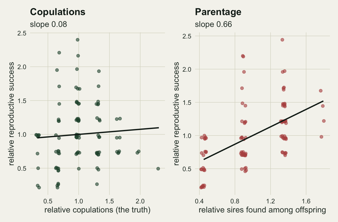
Detected sires cannot outnumber the offspring
The expected number of distinct fathers among n offspring from k equally successful mates is an occupancy count. Each mate is missed by all n offspring with probability (1 - 1/k)^n, so the expectation is k(1 - (1 - 1/k)^n). It is exactly 1 at one offspring, it cannot exceed n, and it approaches k only once n is several times k. That is the whole mechanism in one line: a small brood truncates the mating success it can reveal, and a small brood is also low reproductive success.
exp_sires <- function(n_off, k_mates) k_mates * (1 - (1 - 1 / k_mates)^n_off)

n_draw  <- 20000
off_seq <- 1:16
k_show  <- c(2, 3, 5)
set.seed(2014)
sire_tab <- do.call(rbind, lapply(k_show, function(k_m) {
  do.call(rbind, lapply(off_seq, function(n_o) {
    brood_id <- rep(seq_len(n_draw), each = n_o)
    fathers  <- sample.int(k_m, n_draw * n_o, replace = TRUE)
    pair_key <- unique((brood_id - 1) * k_m + fathers)
    n_dist   <- tabulate((pair_key - 1) %/% k_m + 1, n_draw)
    data.frame(k_mates = k_m, n_off = n_o,
               exact = exp_sires(n_o, k_m), simulated = mean(n_dist),
               se = sd(n_dist) / sqrt(n_draw))
  }))
}))
has_var  <- sire_tab$se > 0
sire_z   <- max(abs(sire_tab$simulated - sire_tab$exact)[has_var] /
                  sire_tab$se[has_var])
n_novar  <- sum(!has_var)
novar_gap <- max(abs(sire_tab$simulated - sire_tab$exact)[!has_var])
k3_n4    <- exp_sires(4, 3)
k3_n8    <- exp_sires(8, 3)
k3_n16   <- exp_sires(16, 3)
k5_n4    <- exp_sires(4, 5)
With 3 mates, a female with 4 offspring shows 2.407 fathers on average, one with 8 shows 2.883, and one with 16 shows 2.995. With 5 mates and 4 offspring the expectation is 2.952, so two extra mates add less than one detected father. The simulated means, 20000 broods per point, sit within 2.4 Monte Carlo standard errors of the formula wherever the simulated count varied. At 5 points it did not vary (one offspring, or a large brood from two mates in which every simulated brood showed both fathers), and there the formula and the simulation differ by at most 0.00006.
ggplot(sire_tab, aes(n_off, exact, colour = factor(k_mates))) +
  geom_abline(slope = 1, intercept = 0, linetype = "dashed",
              colour = te_body, linewidth = 0.5) +
  geom_line(linewidth = 0.9) +
  geom_point(aes(y = simulated), size = 1.8) +
  scale_colour_manual(values = c(te_gold, te_forest, te_rust),
                      name = "true mates") +
  coord_cartesian(ylim = c(0, 5.2)) +
  labs(x = "offspring genotyped", y = "expected fathers detected",
       title = "Small broods hide mates",
       subtitle = "dashed line: detected fathers equal to offspring, the ceiling") +
  theme_datasheet() +
  theme(legend.position = "bottom")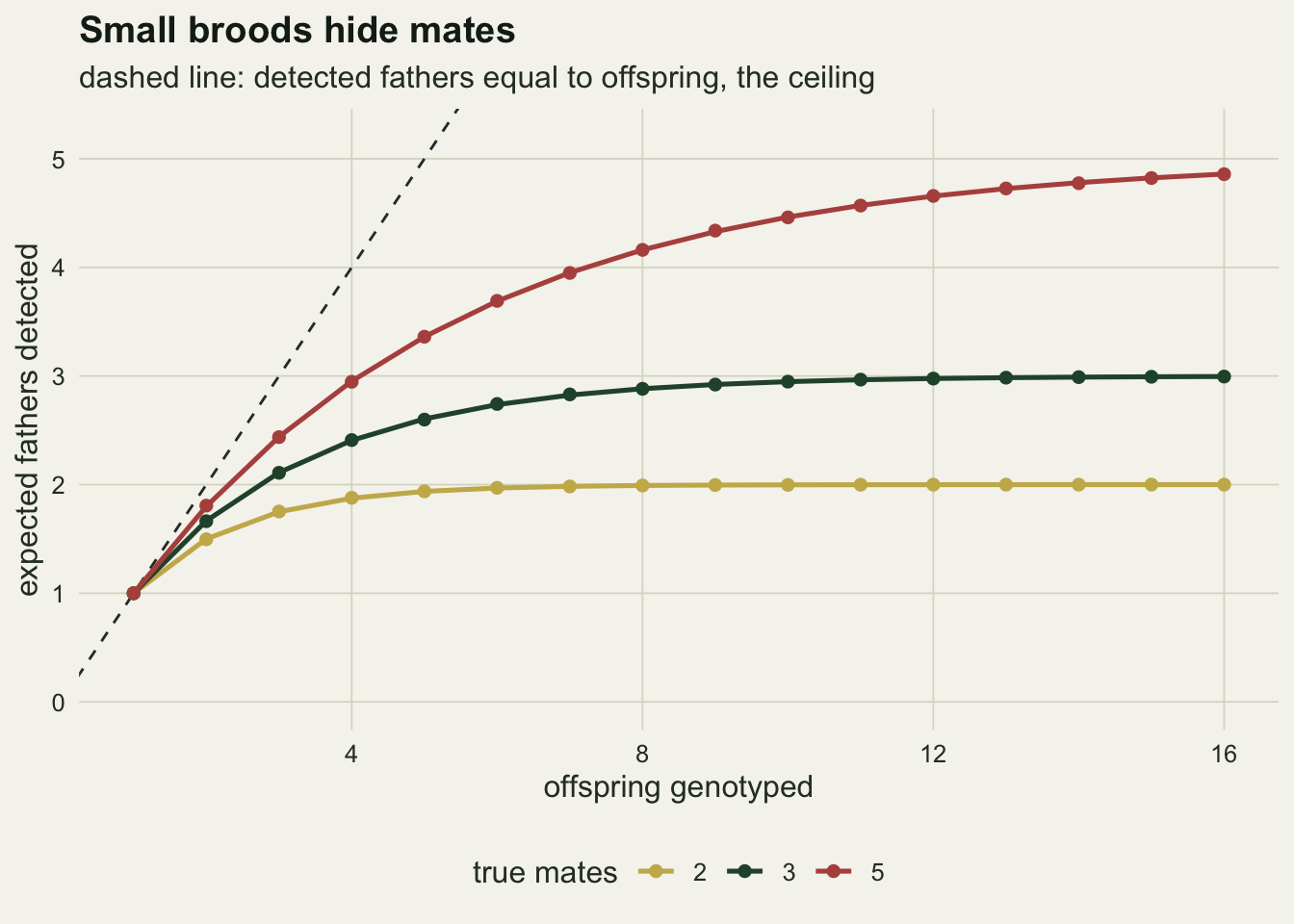
The manufactured gradient across clutch sizes
The grid crosses mean clutch sizes of 2, 4, 8 and 16 with mean mate numbers of 1.5 and 3 and with genotyping of the whole brood or of half of it. Each cell holds 1000 replicate populations of 100 females. That replication was set before the run so that the Monte Carlo standard error of a rejection rate is at most 0.016, and the whole grid takes a few seconds.
n_rep <- 1000
cells <- expand.grid(lambda = c(2, 4, 8, 16), mean_mates = c(1.5, 3),
                     frac = c(1, 0.5))
set.seed(3141)
grid_tab <- do.call(rbind, lapply(seq_len(nrow(cells)), function(j) {
  s_b  <- sim_broods(n_rep, n_fem, cells$lambda[j], cells$mean_mates[j],
                     cells$frac[j])
  g_tr <- gradient_by_rep(s_b$clutch, s_b$mates, s_b$rep_id)
  g_ge <- gradient_by_rep(s_b$typed, s_b$gen_ms, s_b$rep_id)
  g_nz <- gradient_by_rep(s_b$typed, s_b$gen_ms, s_b$rep_id,
                          keep = s_b$typed > 0)
  g_cl <- gradient_by_rep(s_b$clutch, s_b$gen_ms, s_b$rep_id)
  data.frame(cells[j, ],
             true_b  = mean(g_tr$beta_ss), true_sig = mean(g_tr$p_val < 0.05),
             gen_b   = mean(g_ge$beta_ss), gen_se = sd(g_ge$beta_ss) / sqrt(n_rep),
             gen_sig = mean(g_ge$p_val < 0.05),
             nz_b    = mean(g_nz$beta_ss, na.rm = TRUE),
             nz_sig  = mean(g_nz$p_val < 0.05, na.rm = TRUE),
             zero_share = mean(s_b$typed == 0),
             cl_b    = mean(g_cl$beta_ss), cl_sig = mean(g_cl$p_val < 0.05))
}))
mc_se_max <- sqrt(0.25 / n_rep)
cell_of <- function(lam, mm, fr) {
  which(grid_tab$lambda == lam & grid_tab$mean_mates == mm &
          grid_tab$frac == fr)
}
c4  <- cell_of(4, 3, 1);  c8 <- cell_of(8, 3, 1)
c16 <- cell_of(16, 3, 1); c2 <- cell_of(2, 3, 1)
c4l <- cell_of(4, 1.5, 1)
true_range <- range(grid_tab$true_b)
true_sig_range <- range(grid_tab$true_sig)
sig16_se <- sqrt(grid_tab$gen_sig[c16] * (1 - grid_tab$gen_sig[c16]) / n_rep)
p_two_or_less <- ppois(1, 0.5)
Across all 16 cells the gradient on copulation counts averages between -0.005 and 0.004, and its rejection rate at the five per cent level runs from 0.038 to 0.059: the regression on the truth behaves as a test with no effect should.
On parentage with the whole brood genotyped and a mean of 3 mates, the mean gradient is 0.863 at a clutch of 2, 0.560 at 4 (Monte Carlo standard error 0.003), 0.171 at 8, and 0.020 at 16. The share of populations with p below 0.05 is 1.000 at a clutch of 4, 0.543 at 8 and 0.067 at 16, where the Monte Carlo standard error is 0.008 and the excess over five per cent is small but not quite gone. With a mean of 1.5 mates the artefact is smaller, 0.305 at a clutch of 4, because 0.91 of females then have one or two mates and there are fewer fathers for a small brood to hide.
grid_plot <- grid_tab
grid_plot$sampling <- factor(ifelse(grid_plot$frac == 1, "whole brood genotyped",
                                    "half the brood genotyped"),
                             levels = c("whole brood genotyped",
                                        "half the brood genotyped"))
grid_plot$mates_lab <- sprintf("mean mates %.1f", grid_plot$mean_mates)

top_grid <- ggplot(grid_plot, aes(lambda, gen_b, colour = mates_lab)) +
  geom_hline(yintercept = 0, linetype = "dashed", colour = te_body,
             linewidth = 0.5) +
  geom_line(linewidth = 0.9) + geom_point(size = 2.2) +
  facet_wrap(~ sampling) +
  scale_x_log10(breaks = c(2, 4, 8, 16)) +
  scale_colour_manual(values = c(te_gold, te_rust), name = NULL) +
  labs(x = NULL, y = "mean gradient",
       title = "A gradient from nothing",
       subtitle = "dashed line: the true gradient") +
  theme_datasheet() +
  theme(legend.position = "none")

bottom_grid <- ggplot(grid_plot, aes(lambda, gen_sig, colour = mates_lab)) +
  geom_hline(yintercept = 0.05, linetype = "dashed", colour = te_body,
             linewidth = 0.5) +
  geom_line(linewidth = 0.9) + geom_point(size = 2.2) +
  facet_wrap(~ sampling) +
  scale_x_log10(breaks = c(2, 4, 8, 16)) +
  scale_colour_manual(values = c(te_gold, te_rust), name = NULL) +
  labs(x = "mean clutch size", y = "share with p < 0.05",
       subtitle = "dashed line: the nominal five per cent") +
  theme_datasheet() +
  theme(legend.position = "bottom")

(top_grid / bottom_grid) + plot_annotation(theme = theme_datasheet())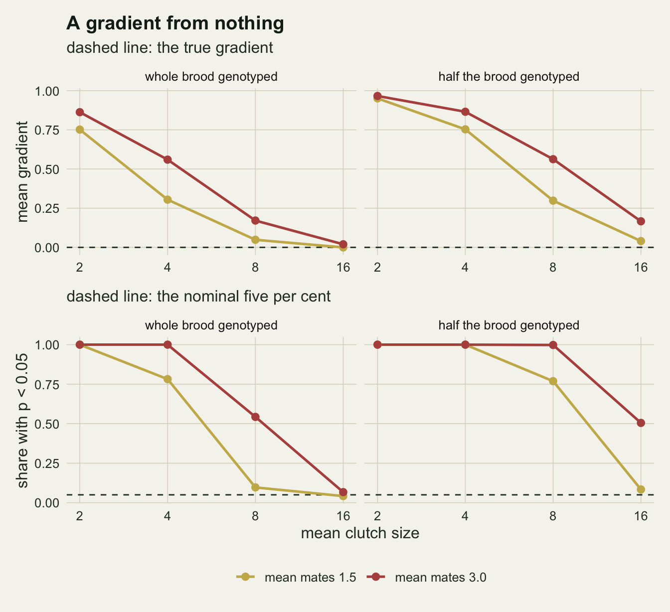
Half the brood is a smaller clutch
Genotyping half of each brood is not a separate problem. A binomial half of a Poisson count with mean 8 is a Poisson count with mean 4, and the fathers of the genotyped offspring are still a fair raffle among the mates. The pair of genotyped offspring and detected fathers therefore has exactly the same distribution in a half-sampled clutch of 8 as in a fully sampled clutch of 4, and the same holds for 16 and 8. The chance that a female contributes no genotyped offspring is exp(-lambda f).
c8h  <- cell_of(8, 3, 0.5)
c16h <- cell_of(16, 3, 0.5)
thin_gap_4 <- grid_tab$gen_b[c8h] - grid_tab$gen_b[c4]
thin_se_4  <- sqrt(grid_tab$gen_se[c8h]^2 + grid_tab$gen_se[c4]^2)
thin_gap_8 <- grid_tab$gen_b[c16h] - grid_tab$gen_b[c8]
thin_se_8  <- sqrt(grid_tab$gen_se[c16h]^2 + grid_tab$gen_se[c8]^2)
gen_se_all <- max(grid_tab$gen_se)
zero_exact_h <- exp(-4 * 0.5)
c4h <- cell_of(4, 3, 0.5)
cl_ratio_8  <- grid_tab$cl_b[c8h] / grid_tab$gen_b[c8h]
cl_ratio_16 <- grid_tab$cl_b[c16h] / grid_tab$gen_b[c16h]
The half-sampled clutch of 8 gives a mean gradient of 0.563 against 0.560 for the whole clutch of 4, a difference of 0.7 standard errors. The half-sampled 16 gives 0.166 against 0.171, 1.3 standard errors apart. At a clutch of 4 with half genotyped, the share of females with no genotyped offspring is 0.1325 against exp(-2) = 0.1353. In the figure each point in the right-hand facets repeats the left-hand point at half its clutch size, which is this arithmetic and nothing more. The practical reading is that a study with large clutches but a genotyping budget of a few offspring per female, and with reproductive success counted as the genotyped offspring, is back in the small-clutch regime.
Many parentage studies count the whole clutch as reproductive success and use the genotyped subsample only for the fathers. The same half-sampled populations can be regressed that way, with the whole clutch as the response and the fathers still counted from half of it. At a half-sampled clutch of 8 the mean gradient is then 0.281 rather than 0.563, significant in a share of 0.969 of populations, and at a half-sampled clutch of 16 it is 0.082 rather than 0.166. The ratios are 0.50 and 0.49: under Poisson thinning the unsampled half is independent of the genotyped half and of the fathers found in it, so the covariance with detected fathers is unchanged while the mean of the response doubles, and the relative slope halves. Smaller, but at a half-sampled clutch of 8 still far from zero.
Dropping the zeros, and a Poisson GLM
Two responses to the artefact are common. The first removes females with no genotyped offspring, since their mating success of zero is plainly an artefact of the counting. The second replaces the least squares slope on relative values with a Poisson regression of offspring on detected mates, on the grounds that the response is a count.
c2l <- cell_of(2, 1.5, 1)
glm_rep <- 200
glm_slope <- function(y_val, x_val) {
  x_mat <- cbind(1, x_val)
  g_fit <- glm.fit(x_mat, y_val, family = poisson())
  mu_f  <- g_fit$fitted.values
  v_cov <- solve(crossprod(x_mat * sqrt(mu_f)))
  z_val <- g_fit$coefficients[2] / sqrt(v_cov[2, 2])
  c(g_fit$coefficients[2], 2 * pnorm(-abs(z_val)))
}
set.seed(2718)
glm_tab <- do.call(rbind, lapply(c(2, 4, 8, 16), function(lam) {
  s_b <- sim_broods(glm_rep, n_fem, lam, 3, 1)
  per_rep <- vapply(seq_len(glm_rep), function(r) {
    in_r <- s_b$rep_id == r
    c(glm_slope(s_b$typed[in_r], s_b$gen_ms[in_r]),
      glm_slope(s_b$clutch[in_r], s_b$mates[in_r]))
  }, numeric(4))
  data.frame(lambda = lam, gen_glm = mean(per_rep[1, ]),
             gen_glm_sig = mean(per_rep[2, ] < 0.05),
             true_glm = mean(per_rep[3, ]),
             true_glm_sig = mean(per_rep[4, ] < 0.05))
}))
g4 <- which(glm_tab$lambda == 4)
g16 <- which(glm_tab$lambda == 16)
clear_cells <- grid_tab$gen_b > 0.1
nz_keep_min <- min(grid_tab$nz_b[clear_cells] / grid_tab$gen_b[clear_cells])
glm_se <- sqrt(0.25 / glm_rep)
Dropping the zero females moves the mean gradient at a clutch of 4 from 0.560 to 0.518, while the share significant stays at 1.000. At a clutch of 4 only 0.019 of females have no offspring, so there is little to drop. The repair does more where zeros are common: at a clutch of 2 with 1.5 mates the gradient falls from 0.752 to 0.495. Across the grid cells where the parentage gradient is above 0.1, dropping the zeros keeps at least 0.66 of it, because the ceiling that matters is not the zero but the one-offspring female with one detected father, and the two-offspring female with at most two.
The Poisson regression, on all females and 200 populations per clutch size, gives a mean log-scale slope per detected father of 0.254 at a clutch of 4, significant in a share of 1.000 of populations (Monte Carlo standard error at most 0.035), against -0.001 and 0.070 on copulation counts. At a clutch of 16 the parentage slope is 0.007, significant in 0.075. The slope is on a different scale from a Bateman gradient, so its size cannot be compared with the least squares value; its sign is the same, and a change of error distribution cannot fix a problem that sits in how the predictor was counted.
A population with a real gradient
The same counting applied where mating does bring offspring gives a different answer. Two versions are simulated. In the first, every mate contributes offspring in proportion, so the expected brood is lambda times the number of mates over the mean number of mates, and the true relative gradient is 1; this is structurally the textbook male case, although it is simulated here as a female brood split among mates. In the second, half of the expected brood is fixed and half scales with mates, so the true gradient is one half.
The first case has a closed form. When a Poisson brood is split by a fair raffle among k mates, each mate’s share is an independent Poisson count with mean mu = lambda / (mean mates). A mate is detected when his share is positive, so given m detected mates the expected brood is m mu / (1 - exp(-mu)). That is a straight line through the origin in m, and when the conditional mean is a line through the origin the population least squares slope on relative values is exactly 1. The mates that parentage misses are precisely the ones that contributed nothing, and leaving them out costs the slope nothing.
set.seed(1673)
real_tab <- do.call(rbind, lapply(c(1, 0.5), function(bnf) {
  do.call(rbind, lapply(c(2, 4, 8, 16), function(lam) {
    s_b  <- sim_broods(n_rep, n_fem, lam, 3, 1, benefit = bnf)
    g_tr <- gradient_by_rep(s_b$clutch, s_b$mates, s_b$rep_id)
    g_ge <- gradient_by_rep(s_b$typed, s_b$gen_ms, s_b$rep_id)
    data.frame(benefit = bnf, lambda = lam,
               true_b = mean(g_tr$beta_ss), gen_b = mean(g_ge$beta_ss),
               gen_se = sd(g_ge$beta_ss) / sqrt(n_rep),
               detect = sum(s_b$gen_ms) / sum(s_b$mates))
  }))
}))
r1_4 <- which(real_tab$benefit == 1 & real_tab$lambda == 4)
r1_2 <- which(real_tab$benefit == 1 & real_tab$lambda == 2)
rh_4 <- which(real_tab$benefit == 0.5 & real_tab$lambda == 4)
rh_16 <- which(real_tab$benefit == 0.5 & real_tab$lambda == 16)
r1_dev <- max(abs(real_tab$gen_b[real_tab$benefit == 1] - 1) /
                real_tab$gen_se[real_tab$benefit == 1])
mu_4 <- 4 / 3
detect_exact_4 <- 1 - exp(-mu_4)
With proportional benefit and a clutch of 4, parentage detects 0.738 of the copulating mates, against 1 - exp(-4/3) = 0.736, and the gradient is 1.001 on parentage against 1.002 on copulations. Across the four clutch sizes the parentage gradient stays within 2.0 standard errors of 1. The two errors, lost mates and the brood ceiling, cancel here, as the formula says they must.
With half the brood independent of mating the cancellation is gone. At a clutch of 4 the parentage gradient is 0.789 against a copulation gradient of 0.504, and at 16 it is 0.513 against 0.502. The fixed part of the brood behaves like the no-benefit population and carries its artefact into the estimate, and the excess shrinks with clutch size as it did in the grid. So the male result in the first case is a property of strict proportionality with equal, Poisson paternity shares, not a general guarantee that a real gradient is safe.
real_long <- rbind(
  data.frame(real_tab[, c("benefit", "lambda")], b = real_tab$true_b,
             source = "copulations"),
  data.frame(real_tab[, c("benefit", "lambda")], b = real_tab$gen_b,
             source = "parentage"))
real_long$panel <- factor(ifelse(real_long$benefit == 1,
                                 "proportional benefit",
                                 "half the brood fixed"),
                          levels = c("proportional benefit",
                                     "half the brood fixed"))
ggplot(real_long, aes(lambda, b, colour = source)) +
  geom_line(linewidth = 0.9) + geom_point(size = 2.2) +
  facet_wrap(~ panel) +
  scale_x_log10(breaks = c(2, 4, 8, 16)) +
  scale_colour_manual(values = c(te_forest, te_rust), name = NULL) +
  coord_cartesian(ylim = c(0.4, 1.1)) +
  labs(x = "mean clutch size", y = "mean Bateman gradient",
       title = "Cancellation is a special case",
       subtitle = "1000 populations of 100 individuals per point") +
  theme_datasheet() +
  theme(legend.position = "bottom")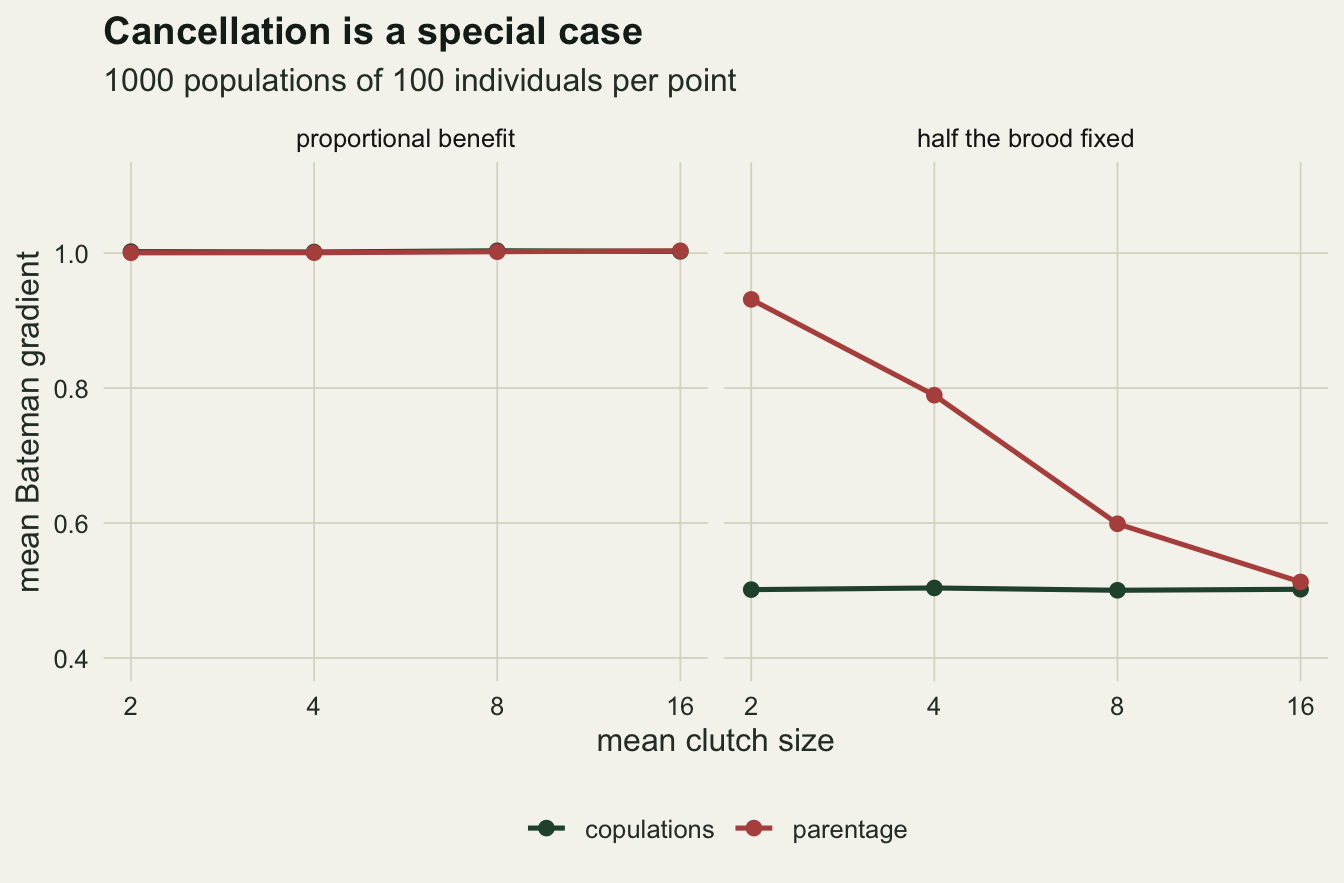
What to report
The opportunity for selection and the opportunity for sexual selection are the other two Bateman metrics, and they carry the same sampling baggage. Under a Poisson brood, the variance over the squared mean of reproductive success is 1 / (lambda f) before any biology enters: it doubles when half the brood is genotyped. The chunk below reads both opportunities, and the Jones (2009) maximum selection differential on mating success (the gradient times the square root of the opportunity for sexual selection), from the no-benefit population at a clutch of 4.
set.seed(918)
opp_pop <- sim_broods(n_rep, n_fem, 4, 3, 1)
rel_var <- function(v, grp) {
  n_g <- tabulate(grp)
  m_v <- rowsum(v, grp)[, 1] / n_g
  (rowsum(v^2, grp)[, 1] / n_g - m_v^2) / m_v^2
}
opp_i     <- mean(rel_var(opp_pop$typed, opp_pop$rep_id))
opp_is_g  <- mean(rel_var(opp_pop$gen_ms, opp_pop$rep_id))
opp_is_t  <- mean(rel_var(opp_pop$mates, opp_pop$rep_id))
opp_b_g   <- mean(gradient_by_rep(opp_pop$typed, opp_pop$gen_ms,
                                  opp_pop$rep_id)$beta_ss)
smax_gen  <- opp_b_g * sqrt(opp_is_g)
opp_b_t   <- mean(gradient_by_rep(opp_pop$clutch, opp_pop$mates,
                                  opp_pop$rep_id)$beta_ss)
smax_true <- opp_b_t * sqrt(opp_is_t)
At a clutch of 4 the opportunity for selection averages 0.246 against 1/4 from the Poisson arithmetic. The opportunity for sexual selection is 0.211 on detected fathers and 0.221 on copulations. The maximum sexual selection differential comes out at 0.257 from parentage and 0.001 from copulations, in a population where mating success buys nothing.
So a parentage-based gradient needs its sampling context printed next to it. Report the mean and the distribution of the number of offspring genotyped per individual, not the clutch size, because the genotyped number sets the ceiling on detected fathers, and state whether reproductive success is the genotyped count or the whole clutch. Report the gradient with and without individuals with no genotyped offspring; Anthes and colleagues (2017) review how the choice of mating success measure and data inclusion decisions shift sexual selection metrics. Simulate the no-benefit null at the observed brood sizes and mate numbers, as the sim_broods function above does in a few lines, and report the observed gradient against that null rather than against zero: at a clutch of 4 and 3 mates the null in this post is not zero but 0.56. Where a comparison between the sexes is the point, compare their brood sizes as well, because a sex difference in the number of offspring per individual produces a sex difference in the artefact.
Honest limits
The null used here is a fair raffle. Real paternity is usually skewed by sperm precedence or cryptic female choice, and a skewed raffle hides minor fathers even in large broods, so the artefact would be expected to fade more slowly with clutch size than the 16-offspring cell suggests. The no-benefit null should be simulated with a paternity skew measured in the study species where one is known, and nothing above measures how much that changes the numbers.
Mating success is assumed to be counted without genotyping error, with every candidate father sampled. Unsampled fathers and assignment errors change the detected count in ways that depend on the pedigree software and the marker panel, and they are outside this simulation.
The copulation count is the simulation’s truth and nothing more. A field study rarely observes all copulations, and a behavioural count has its own undercount (matings out of view) and its own overcount (mounts without sperm transfer). The point of having it here is to separate the artefact from the biology, not to suggest that behavioural data are free of error.
The real-gradient panel covers two specific benefit structures. The exact cancellation under proportional benefit follows from independent Poisson shares; overdispersed broods, or benefits that saturate with mate number, break the line through the origin, and the resulting bias has not been measured here. Neither has the female case Collet and colleagues describe, where males prefer fecund females and a female gradient appears because reproductive success drives mating success rather than the reverse; that is a causal problem a no-benefit null cannot detect.
Only the univariate gradient is examined. Collet and colleagues also argue that the gradient should be partitioned into fecundity and paternity-share components, and the multivariate version is not shown here.
References
Bateman AJ 1948 Heredity 2(3):349-368 (10.1038/hdy.1948.21)
Jones AG 2009 Evolution 63(7):1673-1684 (10.1111/j.1558-5646.2009.00664.x)
Collet JM, Dean RF, Worley K, Richardson DS, Pizzari T 2014 Proceedings of the Royal Society B 281(1782):20132973 (10.1098/rspb.2013.2973)
Anthes N, Haderer IK, Michiels NK, Janicke T 2017 Methods in Ecology and Evolution 8(8):918-931 (10.1111/2041-210X.12707)