Sex ratio evolution and the ESS

Why sex ratios are near 1:1 in R: Fisher’s frequency-dependent argument as an evolutionarily stable strategy, and the female bias under local mate competition.

Most species make roughly equal numbers of sons and daughters, and the reason is one of the oldest arguments in evolutionary biology. It is not that balance is tidy; it is that any imbalance rewards the minority. This is a game, and its solution is an evolutionarily stable strategy. This post builds Fisher’s argument in base R, shows why one half is unbeatable, and then breaks it in the way nature does: local mate competition.

Fisher’s argument as an invasion problem

Every individual has one mother and one father, so the total reproductive success flowing through all sons equals that flowing through all daughters. If sons are rarer than daughters, each son carries a larger share of the next generation, and a parent who makes sons cashes in. Write the fitness of a parent producing a fraction r of sons, in a population whose overall fraction of males is R, as the reproductive value it captures through each sex.

invasion_fitness <- function(r, R) r / (2 * R) + (1 - r) / (2 * (1 - R))
cat(sprintf("population R = 0.5: w(all daughters)=%.3f w(half)=%.3f w(all sons)=%.3f (flat)\n",
            invasion_fitness(0, 0.5), invasion_fitness(0.5, 0.5), invasion_fitness(1, 0.5)))

population R = 0.5: w(all daughters)=1.000 w(half)=1.000 w(all sons)=1.000 (flat)

cat(sprintf("population R = 0.4 (males rare): w(all sons)=%.3f > w(all daughters)=%.3f\n",
            invasion_fitness(1, 0.4), invasion_fitness(0, 0.4)))

population R = 0.4 (males rare): w(all sons)=1.250 > w(all daughters)=0.833

cat(sprintf("population R = 0.6 (males common): w(all sons)=%.3f < w(all daughters)=%.3f\n",
            invasion_fitness(1, 0.6), invasion_fitness(0, 0.6)))

population R = 0.6 (males common): w(all sons)=0.833 < w(all daughters)=1.250

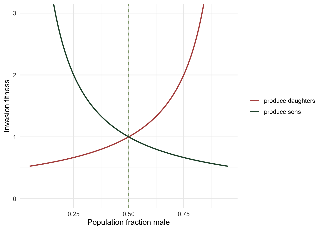
When the population is male-biased at 0.6, making daughters pays 1.250 against 0.833 for sons, so daughter-makers spread and the ratio falls. When it is female-biased at 0.4, the reverse holds and the ratio rises. Only at R = 0.5 does the fitness go flat: producing sons, daughters, or any mix all return exactly 1. A population at one half cannot be invaded by any strategy, which is precisely the definition of an ESS.

One half is the stable point

The crossing is the whole story. Plot the payoff of a son-maker and a daughter-maker as the population ratio slides from all-female to all-male, and they meet at 0.5.

library(ggplot2)
R <- seq(0.05, 0.95, 0.01)
d <- rbind(data.frame(R = R, w = invasion_fitness(1, R), strat = "produce sons"),
           data.frame(R = R, w = invasion_fitness(0, R), strat = "produce daughters"))
ggplot(d, aes(R, w, colour = strat)) +
  geom_vline(xintercept = 0.5, linetype = "dashed", colour = "#93a87f") +
  geom_line(linewidth = 0.9) +
  scale_colour_manual(values = c("produce sons" = "#275139", "produce daughters" = "#b5534e")) +
  coord_cartesian(ylim = c(0, 3)) +
  labs(x = "Population fraction male", y = "Invasion fitness", colour = NULL) +
  theme_minimal(base_size = 12)

Figure 1: Fitness of producing only sons versus only daughters, against the population sex ratio. They cross at 0.5: the rarer sex always pays more, driving the ratio back to equality.

Nothing here mentions what is good for the species; a 1:1 ratio is often wasteful when a few males could fertilise every female. It arises purely from each parent chasing its own advantage, which is why it is a game-theoretic result and not an optimisation for the group.

When one half is wrong: local mate competition

Fisher assumed the whole population mates at random. Hamilton (1967) pointed out that when a few mothers fill a patch and their offspring mate only among themselves before dispersing, sons compete mostly with their own brothers. Extra sons then cannibalise each other’s success, and a mother does better to make daughters. With n foundresses sharing a patch, the ESS fraction of sons is (n - 1) / (2n).

lmc_sons <- function(n) (n - 1) / (2 * n)
cat(sprintf("ESS fraction sons: n=1 %.3f, n=2 %.3f, n=4 %.3f, n=20 %.3f\n",
            lmc_sons(1), lmc_sons(2), lmc_sons(4), lmc_sons(20)))

ESS fraction sons: n=1 0.000, n=2 0.250, n=4 0.375, n=20 0.475

A single foundress should make almost no sons (0 in the limit): one son can fertilise all his sisters. Two foundresses give 0.25, four give 0.375, and as the patch fills with unrelated mothers the ratio climbs back toward Fisher’s one half. Many parasitoid wasps show exactly this pattern, laying strongly female-biased broods when they oviposit alone. The ESS is not a universal 1:1; it is 1:1 only under Fisher’s mixing assumption, and it slides predictably when that assumption fails.

An honest limit

The argument assumes parents can control the sex of their offspring at equal cost, that reproductive value scales simply with rarity, and that population structure is known. Each is a real question in the field: sex determination is often chromosomal and not freely adjustable, sons and daughters can cost different amounts to raise (which shifts the ESS to equal investment, not equal numbers), and the degree of local mate competition is set by dispersal that is hard to observe. Sex allocation is a branch of life-history theory, and like the rest of it, the elegant prediction depends on assumptions the data must earn. The checking post returns to how sensitive these game predictions are to their inputs.

Related tutorials

• The hawk-dove game and the ESS
• The replicator equation
• Checking a game theory model
• Life-history trade-offs

References

Fisher RA 1930. The Genetical Theory of Natural Selection. Oxford: Clarendon Press.

Hamilton WD 1967. Science 156(3774):477-488 (10.1126/science.156.3774.477)

West SA 2009. Sex Allocation. Princeton University Press. ISBN 978-0691089638