The replicator equation in R

Simulate evolutionary game dynamics in base R with the replicator equation: convergence to an ESS, and the rock-paper-scissors cycles that never settle.

Corrected 27 September 2026: the rock-paper-scissors figure shows cycles that slowly widen, which the post presented as sustained cycles without comment; it now explains that the widening is Euler integration error, not biology, and that the printed range is wider than one exact orbit.

An evolutionarily stable strategy tells you where a population can rest, but not whether it ever arrives there, nor what it does if no such rest exists. For that you need dynamics. The replicator equation is the workhorse: it grows each strategy in proportion to how much its payoff exceeds the population mean, and it turns a payoff matrix into a trajectory. This post codes it in base R, confirms it converges on an ESS, and then shows the case that has no ESS at all: rock-paper-scissors.

The equation

For strategy frequencies x and a payoff matrix A, the payoff to strategy i is (A x)_i, the mean payoff is x' A x, and each frequency changes as

\[ \dot{x}_i = x_i\left[(\mathbf{A}\mathbf{x})_i - \mathbf{x}^\top\mathbf{A}\mathbf{x}\right]. \]

A strategy above the average grows, one below it shrinks, and the frequencies always sum to one. Here it is as a plain Euler integrator.

replicator <- function(A, x0, dt = 0.005, tmax = 200) {
  x <- x0; out <- matrix(0, tmax / dt, length(x0))
  for (i in seq_len(nrow(out))) {
    fit <- as.numeric(A %*% x)
    x <- x + dt * x * (fit - sum(x * fit))
    x <- x / sum(x)                      # guard against numerical drift off the simplex
    out[i, ] <- x
  }
  out
}

Rock, paper, scissors: no ESS

The lizard Uta stansburiana runs a real rock-paper-scissors among three male types, where each beats one and loses to another (Sinervo and Lively 1996). Encode the cycle as a zero-sum payoff matrix: winning pays +1, losing -1.

A <- matrix(c( 0, -1,  1,
               1,  0, -1,
              -1,  1,  0), 3, byrow = TRUE)
out <- replicator(A, c(0.5, 0.3, 0.2))
cat(sprintf("time-averaged frequencies: %.3f %.3f %.3f (interior point is 1/3 each)\n",
            mean(out[, 1]), mean(out[, 2]), mean(out[, 3])))

time-averaged frequencies: 0.333 0.336 0.331 (interior point is 1/3 each)

cat(sprintf("strategy 1 ranges over %.3f to %.3f: it never settles\n", min(out[, 1]), max(out[, 1])))

strategy 1 ranges over 0.157 to 0.550: it never settles

The interior point where all three are at 1/3 is an equilibrium, but not an ESS: it is a neutrally stable centre, not an attractor. Started off it, the population orbits forever without converging. The time-average of each strategy is 1/3, yet at no single moment is the population actually there. Reporting “the equilibrium is one-third each” would describe a state the population never occupies.

One thing in the figure below is not biology. The cycles slowly widen over the run: peaks creep up and troughs creep down. For this game the exact orbits are closed, because the product of the three frequencies is conserved, so the widening is error from the simple Euler step, which moves outwards a little on every turn. The range printed above is therefore somewhat wider than a single exact orbit. A smaller dt or a higher-order integrator such as deSolve::ode keeps the amplitude steady.

library(ggplot2)
te_canvas <- theme(plot.background  = element_rect(fill = "#f5f4ee", colour = NA),
                   panel.background = element_rect(fill = "#f5f4ee", colour = NA))
tt <- seq_len(nrow(out)) * 0.005
d <- rbind(data.frame(t = tt, x = out[, 1], s = "rock"),
           data.frame(t = tt, x = out[, 2], s = "paper"),
           data.frame(t = tt, x = out[, 3], s = "scissors"))
ggplot(d, aes(t, x, colour = s)) +
  geom_hline(data = data.frame(y = 1/3), aes(yintercept = y, linetype = "equal frequencies (1/3)"),
             colour = "#93a87f", linewidth = 0.4, inherit.aes = FALSE) +
  geom_line(linewidth = 0.7) +
  scale_colour_manual(values = c(rock = "#275139", paper = "#c9b458", scissors = "#b5534e")) +
  scale_linetype_manual(values = c("equal frequencies (1/3)" = "solid"), name = NULL) +
  labs(x = "Time", y = "Frequency", colour = NULL) +
  theme_minimal(base_size = 12) + te_canvas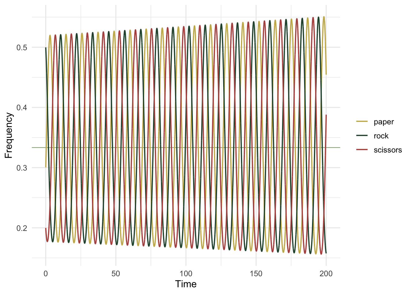

Figure 1: Rock-paper-scissors replicator dynamics. The three frequencies chase each other in sustained cycles and never reach the one-third equilibrium; the mean is 1/3 but the population is never at rest. The slow widening of the cycles is error from the Euler step, not biology.

When it does settle

Not every game cycles. A game with a genuine ESS, like hawk-dove, sends the replicator straight to its stable mix and holds it there. With a resource worth V = 2 and a fight costing C = 3, the ESS is a hawk frequency of V/C = 2/3. Run the same integrator from a population that is almost all doves and from one that is almost all hawks:

V <- 2; C <- 3
H <- matrix(c((V - C) / 2, V,
              0,           V / 2), 2, byrow = TRUE)
for (h0 in c(0.05, 0.95)) {
  hd <- replicator(H, c(h0, 1 - h0))
  cat(sprintf("hawks start at %.2f: %.4f at t = 20, %.4f at t = 200 (V/C = %.4f)\n",
              h0, hd[20 / 0.005, 1], hd[nrow(hd), 1], V / C))
}

hawks start at 0.05: 0.6657 at t = 20, 0.6667 at t = 200 (V/C = 0.6667)
hawks start at 0.95: 0.6678 at t = 20, 0.6667 at t = 200 (V/C = 0.6667)

Both runs converge on the ESS from opposite sides: the hawk frequency is already 0.6657 and 0.6678 by t = 20, and 0.6667 in both at t = 200, which is V/C to four decimal places. The difference is structural: hawk-dove has negative frequency dependence pulling toward a point, while rock-paper-scissors has a rotational flow with nothing at the centre to pull toward. The same equation produces both, so you cannot assume an equilibrium is where a population ends up. Whether an interior point attracts, repels, or merely circles is a question about the flow around it (see basins of attraction), not about the equilibrium alone.

An honest limit

The replicator equation assumes an infinite, well-mixed population reproducing in proportion to payoff, with fixed payoffs and no mutation. Each assumption bends real cases. Finite populations add drift that can push a cycling system to the boundary and lose a strategy for good; spatial structure can stabilise cycles that would otherwise wander; and the payoff matrix is, as ever, assumed rather than measured. The equation is a clear lens on which strategies win and whether they settle, not a literal population forecast. The checking post takes up finite populations and payoff sensitivity directly.

References

Hofbauer J, Sigmund K 2003 Bulletin of the American Mathematical Society 40(4):479-519 (10.1090/S0273-0979-03-00988-1)

Nowak MA, Sigmund K 2004 Science 303(5659):793-799 (10.1126/science.1093411)

Sinervo B, Lively CM 1996 Nature 380(6571):240-243 (10.1038/380240a0)

Related tutorials

• The hawk-dove game and the ESS
• Sex ratio evolution and the ESS
• The Moran process and fixation probability
• Rock-paper-scissors needs local interaction

Reproducibility

• Code last run: 2026-09-30
• R version 4.5.3 (2026-03-11), aarch64-apple-darwin20
• Packages: ggplot2 4.0.3