---
title: "Basins of attraction and the separatrix"
description: "Basins of attraction in R: which starting abundances lead to which stable state, the separatrix that divides them, and why unequal competitors differ."
date: "2026-07-04 14:00"
date-modified: "2026-10-15"
categories: [ecology tutorial, R, community ecology, theoretical ecology, coexistence]
image: thumbnail.png
image-alt: "The abundance plane split into two basins by a separatrix, one basin leading to each species winning."
---
*Corrected 15 October 2026: the introduction said every possible starting point ends in one of the two outcomes, and the thumbnail title said the starts are coloured by winner; a start exactly on the separatrix reaches neither, so the introduction now says almost every start does, and the title says only that the separatrix splits the starts.*
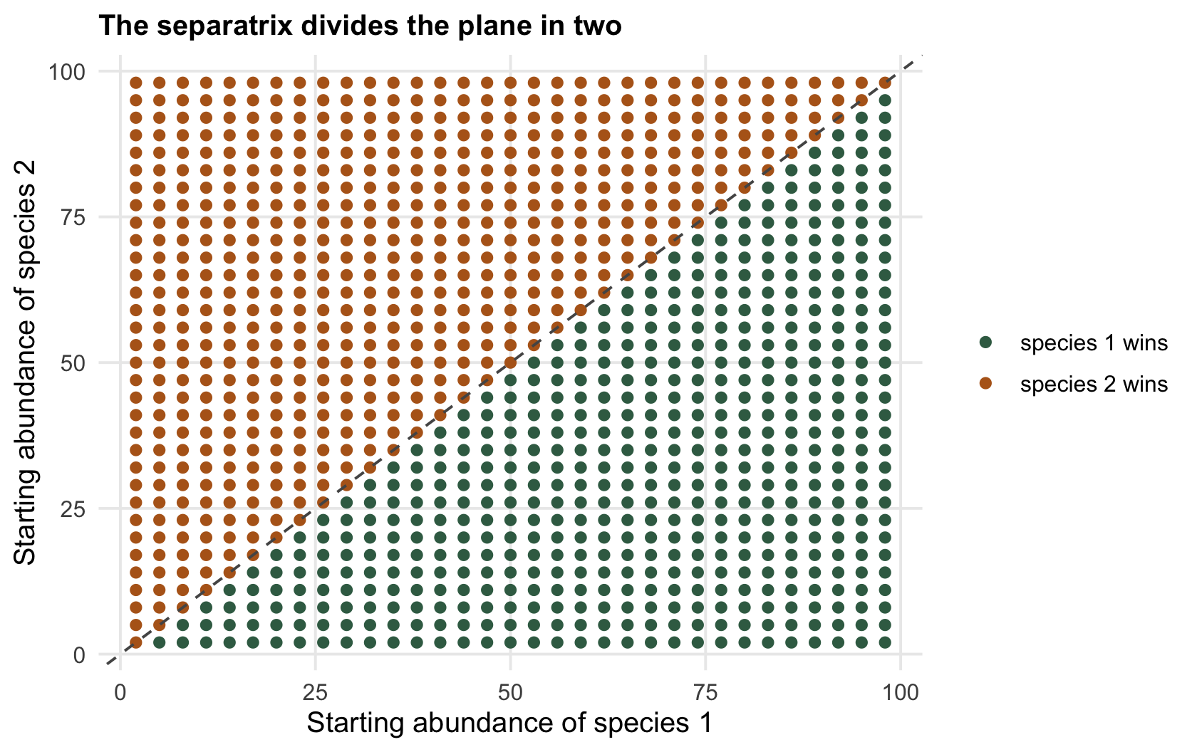
*Corrected 7 October 2026: the caption of the first basin map said every point is coloured by the species that eventually wins; the starts exactly on the diagonal never produce a winner, and the caption now says they take the second species' colour only through the tie rule.*
```{r setup}
#| code-fold: true
#| code-summary: "Setup: packages, colours and plot theme"
#| results: hide
#| message: false
#| warning: false
knitr::opts_chunk$set(echo = TRUE, message = FALSE, warning = FALSE,
                      dev = "png", dpi = 120, fig.path = "figures/",
                      fig.width = 7, fig.height = 4.4)
library(ggplot2)
theme_te <- theme_minimal(base_size = 12) +
  theme(panel.background = element_rect(fill = "#f5f4ee", colour = NA),
        plot.background  = element_rect(fill = "#f5f4ee", colour = NA),
        panel.grid.minor = element_blank(),
        plot.title = element_text(face = "bold", size = 12))
theme_set(theme_te)
col_1 <- "#3a6b52"; col_2 <- "#b5651d"; col_ref <- "#555555"

r1 <- r2 <- 0.5; K1 <- K2 <- 100
winner <- function(N10, N20, a12, a21, Tn = 300, dt = 0.1) {
  N1 <- N10; N2 <- N20
  for (t in 1:(Tn/dt)) {
    dN1 <- r1*N1*(1 - (N1 + a12*N2)/K1); dN2 <- r2*N2*(1 - (N2 + a21*N1)/K2)
    N1 <- max(N1 + dN1*dt, 0); N2 <- max(N2 + dN2*dt, 0)
  }
  if (N1 > N2) 1 else 2
}
grid <- expand.grid(N1 = seq(2, 98, 3), N2 = seq(2, 98, 3))
sym  <- apply(grid, 1, function(x) winner(x[1], x[2], 1.5, 1.5))
asy  <- apply(grid, 1, function(x) winner(x[1], x[2], 1.3, 1.8))   # sp1 the stronger suppressor
frac_sym <- mean(sym == 1); frac_asy <- mean(asy == 1)
Nstar_asy <- c(N1 = K1*(1 - 1.3) / (1 - 1.3*1.8), N2 = K2*(1 - 1.8) / (1 - 1.3*1.8))
```
When a community has [two alternative stable states](../priority-effects-and-alternative-states/), almost every possible starting point belongs to one of two futures: the set of initial abundances that end in species 1 winning, and the set that end in species 2 winning. Those two sets are the basins of attraction, and the surface that divides them is the separatrix; a start exactly on it reaches neither outcome. Mapping the basins turns the vague idea that history matters into a precise picture of exactly which histories lead where.
## Colouring the plane by its outcome
The direct way to find the basins is to take a grid of starting abundances, run each one to its stable state, and record the winner. With equal competitors the map is symmetric.
```{r basins}
r1 <- r2 <- 0.5; K1 <- K2 <- 100
winner <- function(N10, N20, a12, a21, Tn = 300, dt = 0.1) {
  N1 <- N10; N2 <- N20
  for (t in 1:(Tn/dt)) {
    dN1 <- r1*N1*(1 - (N1 + a12*N2)/K1); dN2 <- r2*N2*(1 - (N2 + a21*N1)/K2)
    N1 <- max(N1 + dN1*dt, 0); N2 <- max(N2 + dN2*dt, 0)
  }
  if (N1 > N2) 1 else 2
}
# fraction of a symmetric grid that ends with species 1
mean(apply(expand.grid(N1 = seq(2, 98, 3), N2 = seq(2, 98, 3)), 1,
           function(x) winner(x[1], x[2], 1.5, 1.5)) == 1)
```
With the two species identical, the plane splits in half and the separatrix is the diagonal where the two abundances are equal. The printed fraction falls a little short of a half only because `r sum(grid$N1 == grid$N2)` of the `r nrow(grid)` grid points sit exactly on the diagonal and the rule `if (N1 > N2) 1 else 2` awards every tie to species 2; the points off the diagonal divide exactly evenly. If the species are interchangeable, the only fair boundary is the line that treats them the same. Start with more of species 1 and it wins; start with more of species 2 and it wins; start exactly balanced and you are on the separatrix, the unstable knife-edge itself.
```{r fig-basin}
#| fig-cap: "Basins of attraction for two equal competitors. Each point is a starting pair of abundances, coloured by which species eventually wins; the starts exactly on the diagonal never produce a winner and take the species 2 colour only through the tie rule. The boundary between the basins, the separatrix, is the diagonal of equal abundance."
#| fig-alt: "A scatter of starting points in the abundance plane split into two coloured regions along the diagonal, one region for each species winning."
dg <- cbind(grid, winner = factor(sym, labels = c("species 1 wins", "species 2 wins")))
p_basin <- ggplot(dg, aes(N1, N2, colour = winner)) +
  geom_point(size = 1.7) +
  geom_abline(slope = 1, intercept = 0, colour = col_ref, linetype = "dashed") +
  scale_colour_manual(values = c("species 1 wins" = col_1, "species 2 wins" = col_2)) +
  labs(x = "Starting abundance of species 1", y = "Starting abundance of species 2", colour = NULL,
       title = "The separatrix divides the plane in two")
p_basin
```
```{r}
#| label: thumb
#| include: false
ggsave("thumbnail.png",
p_basin +
labs(title = paste(strwrap("Starting abundances split by the separatrix", 46), collapse = "\n")) +
theme(plot.title = element_text(size = 13, face = "bold"),
plot.subtitle = element_text(size = 9.5),
plot.margin = ggplot2::margin(8, 14, 8, 8)),
width = 7.5, height = 5.4, dpi = 100, bg = "#f5f4ee")
```
## Unequal competitors, unequal basins
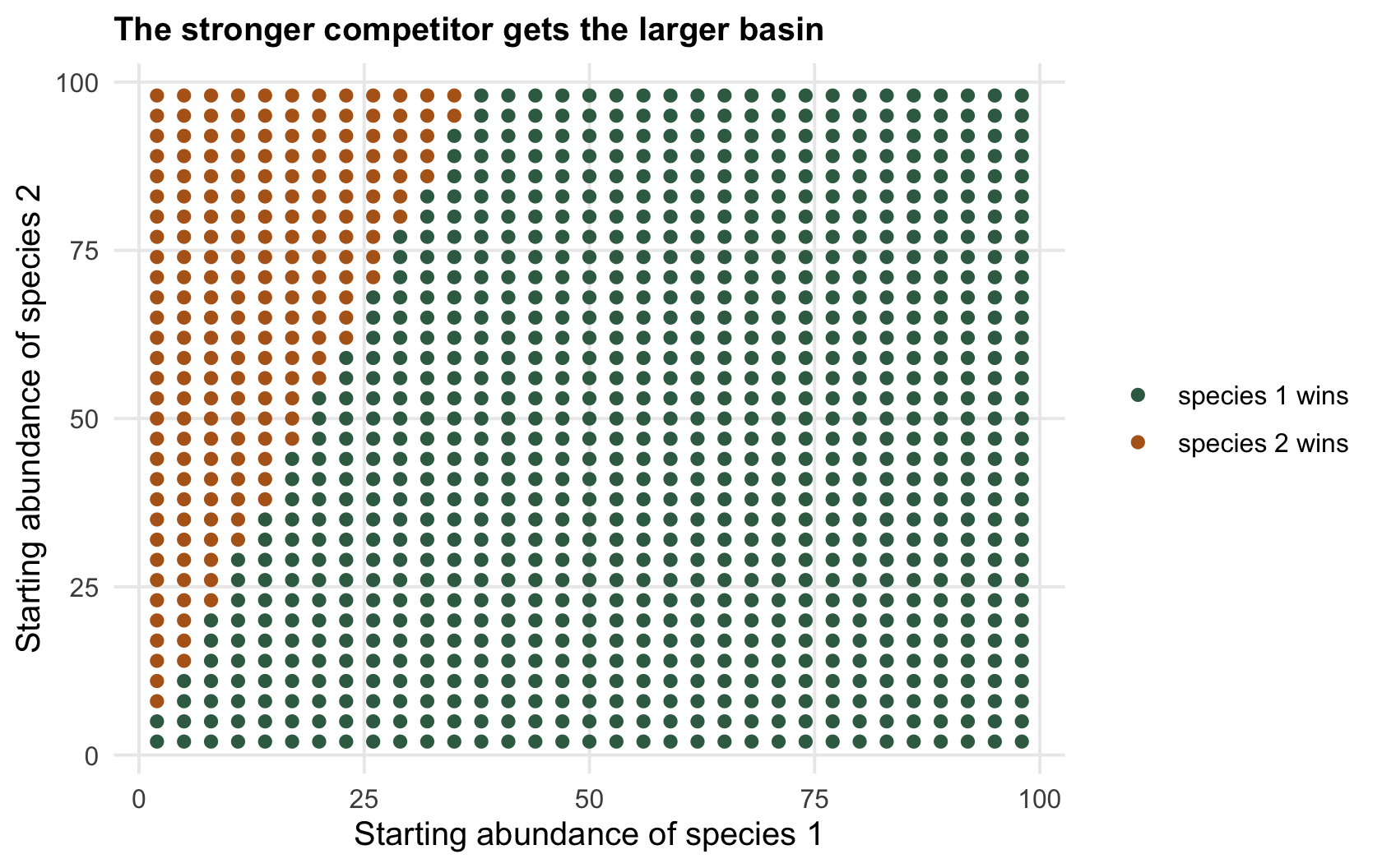
The separatrix only sits on the diagonal when the species are matched. Make one a stronger suppressor of the other and the boundary swings away from it, enlarging its basin: the stronger species wins from a wider range of starts, and needs a smaller head start to do it. Give species 1 the heavier competitive hand and remap.
```{r asymmetric}
# species 1 suppresses species 2 strongly (a21 = 1.8), species 2 suppresses species 1 weakly (a12 = 1.3)
frac1 <- mean(apply(expand.grid(N1 = seq(2, 98, 3), N2 = seq(2, 98, 3)), 1,
                    function(x) winner(x[1], x[2], 1.3, 1.8)) == 1)
round(frac1, 2)
```
Now species 1 wins from `r sprintf("%.0f", frac_asy*100)` per cent of the plane rather than half. It is still a bistable system, species 2 can win, but only from starts where it is well ahead; the unstable point has shifted toward the species 2 axis, to abundances near `r sprintf("%.0f", Nstar_asy["N1"])` and `r sprintf("%.0f", Nstar_asy["N2"])`. This is the quantitative content of a priority effect: a weaker competitor can still win by arriving first, but the window of head starts that lets it do so is narrower the weaker it is.
```{r fig-asym}
#| fig-cap: "Basins when species 1 is the stronger suppressor. Its basin (green) now covers most of the plane; species 2 wins only from starts where it is well ahead. The separatrix has swung toward the species 2 axis."
#| fig-alt: "A scatter of starting points split into two regions, with the green species-1 region much larger than the ochre species-2 region and the boundary shifted off the diagonal."
da <- cbind(grid, winner = factor(asy, labels = c("species 1 wins", "species 2 wins")))
ggplot(da, aes(N1, N2, colour = winner)) +
  geom_point(size = 1.7) +
  scale_colour_manual(values = c("species 1 wins" = col_1, "species 2 wins" = col_2)) +
  labs(x = "Starting abundance of species 1", y = "Starting abundance of species 2", colour = NULL,
       title = "The stronger competitor gets the larger basin")
```
## What the basin map tells you
A basin map is the honest answer to "does history matter here, and how much?" A separatrix wedged into one corner means the system is almost monostable: only extreme starts reach the small basin, and in practice the community nearly always ends up the same way. A separatrix near the diagonal means the outcome is genuinely up for grabs, sensitive to small differences in who arrives first and in what numbers. For restoration and management this is the practical quantity: not just whether an alternative state exists, but how large a push toward it is needed, which is the width of the basin you have to cross. That push, followed along a single changing driver rather than the starting abundances, is the [tipping point](../hysteresis-and-tipping-points/), and the difficulty of confirming any of it from field data is the [checking post](../checking-for-alternative-stable-states/).
## References
- Lewontin RC 1969. Brookhaven Symposia in Biology 22:13-24.
- Beisner BE, Haydon DT, Cuddington K 2003. Frontiers in Ecology and the Environment 1(7):376-382 (10.1890/1540-9295(2003)001[0376:ASSIE]2.0.CO;2).
## Related tutorials
- [Priority effects and alternative stable states](../priority-effects-and-alternative-states/)
- [Hysteresis and tipping points](../hysteresis-and-tipping-points/)
- [Checking for alternative stable states](../checking-for-alternative-stable-states/)
- [The replicator equation](../the-replicator-equation/)