Checking for alternative stable states

Testing alternative stable states in R: why a bimodal distribution is not proof, why a driver mimics one, and how perturbation and hysteresis give the evidence.

Alternative stable states are one of the most consequential ideas in ecology and one of the hardest to prove. The trouble is that the pattern they leave, a system that sits in one of two very different conditions, is also produced by things that are not alternative stable states at all: a sharp response to an environmental gradient, a threshold in a driver, plain measurement of two different places. A field data set almost never comes with the manipulation that would settle the question, so most claims rest on patterns that have innocent explanations. These three checks are what a claim of alternative stable states has to survive.

Check 1: a bimodal distribution is not bistability

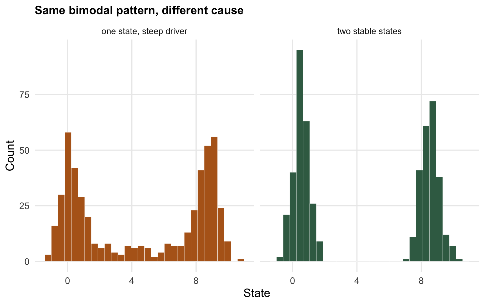
The most common evidence offered is a histogram with two peaks: many sites are either high or low, few in between, so surely there are two states. But a single-valued response to a driver produces exactly the same histogram. If a system tracks one stable state that happens to change steeply with some environmental variable, then even an evenly sampled driver piles the states up at two values with a gap in the middle, because the steep part of the response covers only a sliver of the gradient and few sites are caught in it, and none of that is bistability.

set.seed(169)
env <- runif(500, 0, 4)
state_mono <- 9/(1 + exp(4*(env - 2))) + rnorm(500, 0, 0.5)   # ONE state, steep function of a driver
state_bi   <- ifelse(rbinom(500, 1, 0.5) == 1, 8.5, 0.6) + rnorm(500, 0, 0.5)  # TWO states
c(mono_gap = mean(state_mono > 2 & state_mono < 6),   # both are bimodal: few in the middle
  bi_gap   = mean(state_bi   > 2 & state_bi   < 6))

mono_gap   bi_gap 
   0.098    0.000 

Both distributions are bimodal, and what separates them is a matter of degree: the driver-generated one still leaves about a tenth of the sites in the middle, while the truly bistable one leaves that band empty. One comes from a single state bent steeply by a driver, the other from genuine bistability, and the histogram barely distinguishes them. A slightly steeper driver, or a little less measurement noise, would close the remaining gap as well. A bimodal distribution is a starting point for a question, never an answer to it.

db <- rbind(data.frame(x = state_mono, src = "one state, steep driver"),
            data.frame(x = state_bi,   src = "two stable states"))
ggplot(db, aes(x, fill = src)) +
  geom_histogram(bins = 30, colour = "white", linewidth = 0.1) +
  facet_wrap(~src) +
  scale_fill_manual(values = c("one state, steep driver" = col_b, "two stable states" = col_a), guide = "none") +
  labs(x = "State", y = "Count", title = "Same bimodal pattern, different cause") +
  theme(strip.text = element_text(size = 9))

Figure 1: Two state distributions, both bimodal. The left comes from a single stable state responding steeply to a driver; the right from true bistability. The left keeps a thin scatter of sites between the peaks and the right does not, but the shapes are close enough that bimodality alone decides nothing.

Check 2: does a driver explain the two groups?

The first thing to try is cheap: see whether a measured driver accounts for which state each site is in. If it does, the parsimonious reading is a threshold response, not two states; if the states are unrelated to every driver you can measure, alternative stable states become more plausible. It is a screen, not a proof, but it removes the easy explanations.

c(driver_explains_mono = round(cor(env, state_mono), 2),
  driver_explains_bi   = round(cor(env, state_bi),   2))

driver_explains_mono   driver_explains_bi 
               -0.94                -0.01 

In the single-state data the driver and the state are tightly related, a correlation of -0.94: the environment tells you almost exactly which mode a site is in, so there is no need to invoke two states. In the bistable data the same driver is essentially uncorrelated with the state, -0.01: sites in opposite states sit at the same environmental value. That is the signature worth chasing, though it is still not conclusive, because an unmeasured driver could always be doing the work of the one you measured.

Check 3: the perturbation and the hysteresis

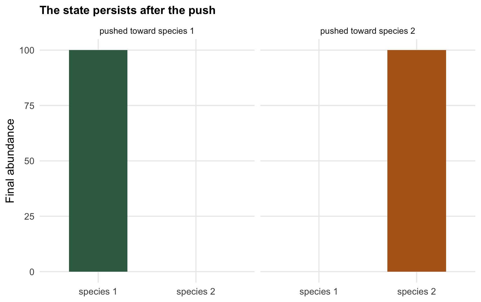
The only decisive evidence is dynamical, and it takes a manipulation. Alternative stable states make a specific promise: push the system hard enough to cross the boundary and it stays in the new state after the push ends, under the same conditions as before. A monostable system, perturbed, slides back. So the definitive test is to displace the system and watch whether it returns or holds. In the bistable model, starting the community on either side of the separatrix sends it to a different, permanent state.

# same parameters, two starting points either side of the boundary: the state that persists differs
rbind(pushed_toward_2 = run_lv(c(30, 70)),
      pushed_toward_1 = run_lv(c(70, 30)))

                [,1] [,2]
pushed_toward_2    0  100
pushed_toward_1  100    0

A community displaced toward species 2 settles at (0, 100) and stays there; displaced toward species 1 it settles at (100, 0) and stays there. The persistence of the new state after the perturbation is removed is the thing a single stable state cannot do, and it is what the classic field experiments on rocky shores and lakes were designed to show. The comparable signature along a driver is hysteresis: if pushing the driver up collapses the system at one value and pulling it back only restores it at a much lower value, the loop is hard to explain without two states. Both tests need the system to be driven, not just observed.

dp <- rbind(data.frame(perturbation = "pushed toward species 2", sp = c("species 1", "species 2"), N = push_hi),
            data.frame(perturbation = "pushed toward species 1", sp = c("species 1", "species 2"), N = push_lo))
ggplot(dp, aes(sp, N, fill = sp)) +
  geom_col(width = 0.6) + facet_wrap(~perturbation) +
  scale_fill_manual(values = c("species 1" = col_a, "species 2" = col_b), guide = "none") +
  labs(x = NULL, y = "Final abundance", title = "The state persists after the push") +
  theme(strip.text = element_text(size = 9))

Figure 2: A perturbation test. Displaced across the boundary toward one species or the other, the community settles into a different state and stays: the state depends on the perturbation, not just the conditions, which a single stable state cannot do.

The weight of the evidence

Three checks, and they climb a ladder of difficulty. Bimodality is free and proves nothing; a driver screen is cheap and can rule out the easy alternatives; only a perturbation or a demonstrated hysteresis loop, both of which need the system actually manipulated, can carry the claim. This is why rigorously confirmed alternative stable states in nature are far rarer than the idea’s popularity suggests, and why careful reviews keep returning most field examples to the “suggestive, not established” pile. None of this is an argument that alternative stable states are unreal; the theory is sound and the best experimental cases are convincing. It is an argument that the bar is a manipulation, and that a bimodal histogram from a snapshot survey, however striking, has not cleared it.

References

• Schroder A, Persson L, De Roos AM 2005. Oikos 110(1):3-19 (10.1111/j.0030-1299.2005.13962.x).
• Petraitis PS, Latham RE 1999. Ecology 80(2):429-442 (10.1890/0012-9658(1999)080[0429:TIOSIT]2.0.CO;2).

Related tutorials

• Priority effects and alternative stable states
• Basins of attraction
• Hysteresis and tipping points
• Checking an Allee analysis