---
title: "Hysteresis and tipping points"
description: "Tipping points in R: how a slow driver pushes an ecosystem past a fold, why the collapse is sudden, and why simply reversing the driver does not reverse it."
date: "2026-07-04 15:00"
categories: [ecology tutorial, R, theoretical ecology, population models, community ecology]
image: thumbnail.png
image-alt: "A folded equilibrium curve where a system on the upper branch collapses at one driver value and only recovers at a much lower one."
---
```{r setup}
#| code-fold: true
#| code-summary: "Setup: packages, colours and plot theme"
#| results: hide
#| message: false
#| warning: false
knitr::opts_chunk$set(echo = TRUE, message = FALSE, warning = FALSE,
                      dev = "png", dpi = 120, fig.path = "figures/",
                      fig.width = 7, fig.height = 4.4)
library(ggplot2)
theme_te <- theme_minimal(base_size = 12) +
  theme(panel.background = element_rect(fill = "#f5f4ee", colour = NA),
        plot.background  = element_rect(fill = "#f5f4ee", colour = NA),
        panel.grid.minor = element_blank(),
        plot.title = element_text(face = "bold", size = 12))
theme_set(theme_te)
col_up <- "#3a6b52"; col_dn <- "#b5651d"; col_ref <- "#555555"; col_un <- "#8aa29e"

r <- 1; K <- 10; h <- 1
growth <- function(x) r*x*(1 - x/K); graze <- function(x, c) c*x^2/(x^2 + h^2)
# equilibrium curve via inversion: c(x) = growth(x) / (x^2/(x^2+h^2))
xg <- seq(0.02, K, 0.002); cg <- growth(xg) / (xg^2/(xg^2 + h^2))
# fold points: turning points of c(x)
dcg <- diff(cg); turn <- which(diff(sign(dcg)) != 0)
folds_c <- sort(cg[turn + 1]); c_recover <- folds_c[1]; c_collapse <- folds_c[2]
# hysteresis sweep
sim_eq <- function(c, x0, Tn = 400, dt = 0.05) { x <- x0; for (t in 1:(Tn/dt)) x <- max(x + (growth(x) - graze(x, c))*dt, 0); x }
cs <- seq(1.4, 3.0, 0.02)
up <- numeric(length(cs)); x <- 9; for (i in seq_along(cs)) { x <- sim_eq(cs[i], x); up[i] <- x }
dn <- numeric(length(cs)); x <- 0.3; for (i in rev(seq_along(cs))) { x <- sim_eq(cs[i], x); dn[i] <- x }
veg_at2 <- up[which.min(abs(cs - 2))]; col_at2 <- dn[which.min(abs(cs - 2))]
window_w <- c_collapse - c_recover
```
A lake stays clear for decades as nutrient input creeps up, then turns green almost overnight. A grassland holds against grazing until one more animal tips it into bare soil. What makes these shifts alarming is not only that they are sudden but that they are sticky: undo the pressure that caused them and the system does not simply slide back. This is a tipping point with hysteresis, and it comes from the same folded structure that gives a community [alternative stable states](../priority-effects-and-alternative-states/), seen now along a single slowly changing driver.
## A fold in the equilibrium curve
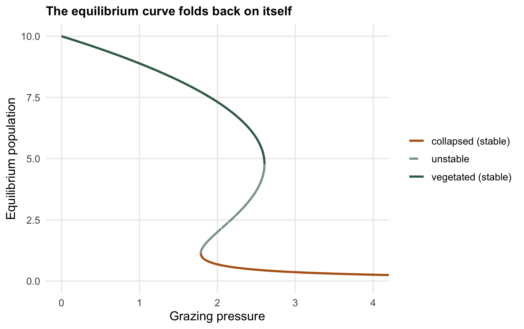
Take a population with logistic growth that also suffers a loss with a saturating, threshold-like shape: grazing that is gentle when the population is sparse, bites hardest at intermediate density, and saturates when the grazers are full. Plot the equilibrium population against the grazing pressure by asking, for each population level, what pressure would hold it steady. The answer is not a single falling line; it folds back on itself.
```{r equilibrium}
r <- 1; K <- 10; h <- 1
growth <- function(x) r*x*(1 - x/K)          # logistic growth
graze  <- function(x, c) c*x^2/(x^2 + h^2)   # saturating, threshold-shaped loss
xg <- seq(0.02, K, 0.002)
cg <- growth(xg) / (xg^2/(xg^2 + h^2))          # grazing pressure that holds each x steady
c(lower_fold = round(sort(cg[which(diff(sign(diff(cg))) != 0) + 1])[1], 2),
  upper_fold = round(sort(cg[which(diff(sign(diff(cg))) != 0) + 1])[2], 2))
```
The equilibrium curve has two folds, at grazing pressures of `r sprintf("%.2f", c_recover)` and `r sprintf("%.2f", c_collapse)`. Between them the curve has three arms: a high, vegetated branch and a low, collapsed branch, both stable, separated by a middle arm that is unstable and cannot be occupied. Outside that window there is only one equilibrium, high to the left, low to the right. The folded middle is where a system can be in either of two states under exactly the same conditions.
```{r fig-fold}
#| fig-cap: "The equilibrium population against grazing pressure. The upper (vegetated) and lower (collapsed) branches are stable; the middle branch is unstable. Between the two folds the system has two possible states."
#| fig-alt: "A folded S-shaped curve of equilibrium population against a driver, with solid upper and lower branches and a dashed unstable middle branch between two fold points."
# classify each branch by its position relative to the two fold x-values
xfold <- xg[which(diff(sign(diff(cg))) != 0) + 1]
branch <- ifelse(xg < min(xfold), "collapsed (stable)",
          ifelse(xg > max(xfold), "vegetated (stable)", "unstable"))
dfold <- data.frame(c = cg, x = xg, branch = branch)
ggplot(dfold, aes(c, x, colour = branch, linetype = branch, group = branch)) +
  geom_line(linewidth = 1) +
  scale_colour_manual(values = c("vegetated (stable)" = col_up, "collapsed (stable)" = col_dn, "unstable" = col_un)) +
  scale_linetype_manual(values = c("vegetated (stable)" = 1, "collapsed (stable)" = 1, "unstable" = 2)) +
  coord_cartesian(xlim = c(0, 4), ylim = c(0, 10)) +
  labs(x = "Grazing pressure", y = "Equilibrium population", colour = NULL, linetype = NULL,
       title = "The equilibrium curve folds back on itself")
```
## Push it up, bring it down: the loop
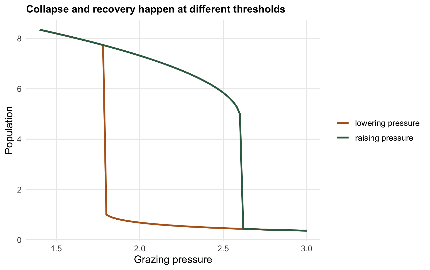
Now change the driver slowly and let the population follow. Start vegetated and raise the grazing pressure: the population eases down the upper branch, holding on until the pressure reaches the upper fold, where the branch simply ends and the system falls to the collapsed state. Then lower the pressure again. It does not climb back at the same point; it stays collapsed until the pressure drops all the way to the lower fold before it recovers. The path up and the path down do not match, and the gap between them is hysteresis.
```{r sweep}
# run the population to near-equilibrium at a given pressure, starting from x0
sim_eq <- function(c, x0, Tn = 400, dt = 0.05) {
  x <- x0
  for (t in 1:(Tn/dt)) x <- max(x + (growth(x) - graze(x, c))*dt, 0)
  x
}
cs <- seq(1.4, 3.0, 0.02)
up <- numeric(length(cs)); x <- 9                                         # raise pressure
for (i in seq_along(cs)) { x <- sim_eq(cs[i], x); up[i] <- x }
dn <- numeric(length(cs)); x <- 0.3                                       # lower pressure
for (i in rev(seq_along(cs))) { x <- sim_eq(cs[i], x); dn[i] <- x }
veg_at2 <- up[which.min(abs(cs - 2))]; col_at2 <- dn[which.min(abs(cs - 2))]
```
```{r fig-loop}
#| fig-cap: "A slow round trip in grazing pressure. Raising it (green) holds the vegetated state until the upper fold, then collapse; lowering it (ochre) stays collapsed until the lower fold, then recovery. The two paths differ: hysteresis."
#| fig-alt: "A hysteresis loop of population against grazing pressure; the increasing-pressure path collapses at a high driver value and the decreasing-pressure path recovers at a lower one, leaving a gap."
dl <- rbind(data.frame(c = cs, x = up, dir = "raising pressure"),
            data.frame(c = cs, x = dn, dir = "lowering pressure"))
ggplot(dl, aes(c, x, colour = dir)) +
  geom_line(linewidth = 1) +
  scale_colour_manual(values = c("raising pressure" = col_up, "lowering pressure" = col_dn)) +
  labs(x = "Grazing pressure", y = "Population", colour = NULL,
       title = "Collapse and recovery happen at different thresholds")
```
At a grazing pressure of `r sprintf("%.1f", 2)`, squarely inside the window, the system can hold `r sprintf("%.1f", veg_at2)` if it arrived from the vegetated side or sit at `r sprintf("%.1f", col_at2)` if it arrived from the collapsed side: same pressure, two states, set by history. Collapse waits until pressure `r sprintf("%.2f", c_collapse)`, but recovery does not come until pressure falls back to `r sprintf("%.2f", c_recover)`, a width of `r sprintf("%.2f", window_w)` that you have to give back and then some. This is why tipping points are dangerous in a way that gradual change is not: the warning is quiet, the collapse is fast, and the repair costs far more than the damage did.
## Reading it in the real world
The practical lessons of the fold are sobering. Because the upper branch stays smooth almost until it ends, the state of a system is a poor guide to how close it is to tipping; a lake or a rangeland can look healthy right up to the edge. Because recovery needs the driver pushed well past the point where collapse happened, restoring the original conditions is often not enough, and managers who reduce nutrients or grazing back to "before" levels can be puzzled when nothing recovers. And because the collapsed state is genuinely stable, it resists the small interventions that would have prevented it. The one piece of good news is that folds can leave statistical fingerprints as they approach, a slowing of recovery from small disturbances, which is one of the few early warnings available, though a fragile one. Confirming that a real system even has this structure, rather than just responding smoothly to its environment, is the hard problem of the [checking post](../checking-for-alternative-stable-states/).
## References
- May RM 1977. Nature 269(5628):471-477 (10.1038/269471a0).
- Scheffer M, Carpenter S, Foley JA, Folke C, Walker B 2001. Nature 413(6856):591-596 (10.1038/35098000).
## Related tutorials
- [Priority effects and alternative stable states](../priority-effects-and-alternative-states/)
- [Basins of attraction](../basins-of-attraction/)
- [Checking for alternative stable states](../checking-for-alternative-stable-states/)
- [The paradox of enrichment in R](../the-paradox-of-enrichment/)