Checking a game theory model

Three checks for evolutionary game models in R: sensitivity to assumed payoffs, drift around an ESS in finite populations, and when the ESS is never reached.

An evolutionarily stable strategy is a clean answer to a clean question, and the danger is trusting the answer past the assumptions that produced it. Three of those assumptions fail routinely in ecology: that the payoffs are known, that the population is infinite, and that the dynamics actually reach the stable point. This post checks each in base R.

Check 1: the ESS is only as good as the payoffs

The hawk-dove ESS is the fraction of hawks V/C, and both V and C are quantities a modeller supplies. A field study almost never measures the fitness cost of an injury on the same scale as the value of a contested resource, so the input is a guess, and the output inherits its uncertainty.

ess_hawks <- function(V, C) V / C
grid <- expand.grid(V = c(2, 3, 4), C = c(5, 8))
grid$ess <- with(grid, ess_hawks(V, C))
grid

  V C   ess
1 2 5 0.400
2 3 5 0.600
3 4 5 0.800
4 2 8 0.250
5 3 8 0.375
6 4 8 0.500

The stable mix ranges from 0.25 to 0.80 across payoff values that are all biologically plausible. A model that reports “40% hawks” without reporting how hard that number leans on the assumed cost is selling false precision. The honest output is a range across the payoffs the data cannot pin down.

Check 2: finite populations drift around the ESS

The replicator equation assumes an infinite population, so the ESS is an exact resting point. Real populations are finite, and sampling each generation adds drift. Simulate a Wright-Fisher population playing hawk-dove, started at the ESS, and watch it wander.

V <- 2; C <- 5; pstar <- V / C
hawk_pay <- function(p) p * ((V - C) / 2) + (1 - p) * V
dove_pay <- function(p) p * 0 + (1 - p) * (V / 2)
wf_run <- function(N, gens = 200, beta = 0.6) {
  p <- pstar
  for (g in seq_len(gens)) {
    wh <- exp(beta * hawk_pay(p)); wd <- exp(beta * dove_pay(p))
    p <- rbinom(1, N, p * wh / (p * wh + (1 - p) * wd)) / N
  }
  p
}
set.seed(438)
for (N in c(200, 100, 50)) {
  fin <- replicate(3000, wf_run(N))
  cat(sprintf("N = %3d: mean hawk frequency = %.3f, SD = %.3f\n", N, mean(fin), sd(fin)))
}

N = 200: mean hawk frequency = 0.398, SD = 0.045
N = 100: mean hawk frequency = 0.397, SD = 0.066
N =  50: mean hawk frequency = 0.392, SD = 0.095

The mean stays glued to the ESS of 0.4, because negative frequency dependence keeps pulling the population back. But the spread grows as the population shrinks: a standard deviation of 0.045 at 200 individuals becomes 0.095 at 50. In a small population the “stable strategy” is a cloud, not a point, and over long enough times drift can push a strategy out entirely. The deterministic ESS predicts the centre; it says nothing about the width, and the width is what a small population lives in.

library(ggplot2)
set.seed(438)
dd <- do.call(rbind, lapply(c(200, 100, 50), function(N)
  data.frame(p = replicate(3000, wf_run(N)), N = factor(N, levels = c(200, 100, 50)))))
ggplot(dd, aes(p, fill = N)) +
  geom_vline(xintercept = pstar, colour = "#46604a", linewidth = 0.4) +
  geom_density(alpha = 0.5, colour = NA) +
  scale_fill_manual(values = c("200" = "#275139", "100" = "#c9b458", "50" = "#b5534e")) +
  labs(x = "Hawk frequency after 200 generations", y = "Density", fill = "N") +
  theme_minimal(base_size = 12) + theme(legend.position = "top")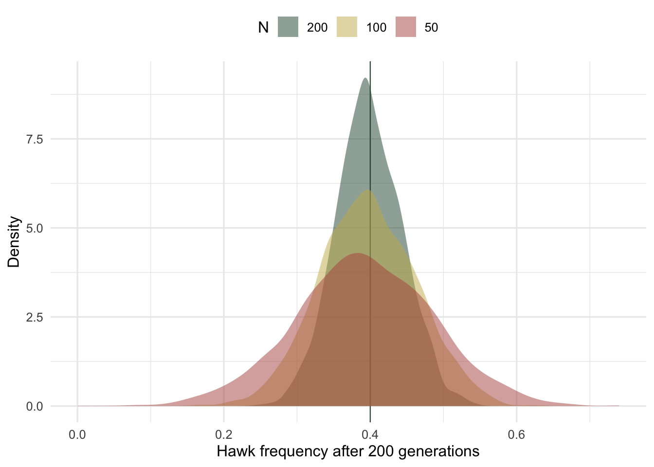

Figure 1: Hawk frequency after 200 generations, started at the ESS of 0.4, for three population sizes. Selection holds the mean at the ESS while drift widens the distribution as N falls.

Check 3: an ESS need not be reached

An ESS is defined by resistance to invasion once common, which says nothing about whether a population starting elsewhere gets there. When a game has two stable strategies, the outcome depends on where you begin. Take a coordination game with an unstable interior equilibrium at 0.25.

replicator2 <- function(payA, payB, x0, dt = 0.01, tmax = 80) {
  x <- x0
  for (i in seq_len(tmax / dt)) {
    f1 <- payA * x; f2 <- payB * (1 - x)
    x <- x + dt * x * (f1 - (x * f1 + (1 - x) * f2)); x <- min(max(x, 0), 1)
  }
  x
}
a <- 3; b <- 1
cat(sprintf("unstable threshold at x* = b/(a+b) = %.2f\n", b / (a + b)))

unstable threshold at x* = b/(a+b) = 0.25

cat(sprintf("start 0.20 -> %.2f    start 0.30 -> %.2f    (same game, opposite fates)\n",
            replicator2(a, b, 0.20), replicator2(a, b, 0.30)))

start 0.20 -> 0.00    start 0.30 -> 1.00    (same game, opposite fates)

The same game sends a population starting at 0.20 to one strategy and a population starting at 0.30 to the other. Which ESS wins is set by history, not by the payoffs alone, exactly the founder effect that produces alternative stable states (see basins of attraction). Rock-paper-scissors is the sharper version: it has an interior equilibrium that is not an ESS and that the dynamics never reach, only circle. Reporting “the ESS” as the prediction is safe only after checking that the dynamics can actually arrive at it.

The assumption underneath

All three checks point at the same thing: a game model is an argument about payoffs, and the payoffs are assumed, not measured. The ESS is a rigorous consequence of a matrix that field data rarely deliver, so the model earns its keep as a way to reason about which strategies can persist and why, not as a numerical forecast of strategy frequencies in a named population. Treat the ESS as a hypothesis about the direction of selection, report how it moves as the payoffs and population size change, and it stays honest.

Related tutorials

• The hawk-dove game and the ESS
• The replicator equation
• Checking a spatial cooperation model
• Neutral theory and the Ewens formula

References

Maynard Smith J 1982. Evolution and the Theory of Games. Cambridge University Press. ISBN 978-0521288842

Nowak MA, Sasaki A, Taylor C, Fudenberg D 2004. Nature 428(6983):646-650 (10.1038/nature02414)

Nowak MA, Sigmund K 2004. Science 303(5659):793-799 (10.1126/science.1093411)