---
title: "Checking a spatial cooperation model"
description: "Four diagnostics for lattice models of cooperation in R: update timing, neighbourhood and boundary choices, seed replication, and whether the game matters."
date: "2026-07-09 11:00"
date-modified: "2026-10-14"
categories: [evolutionary ecology, evolutionary game theory, model diagnostics, spatial ecology, R, ecology tutorial]
image: thumbnail.png
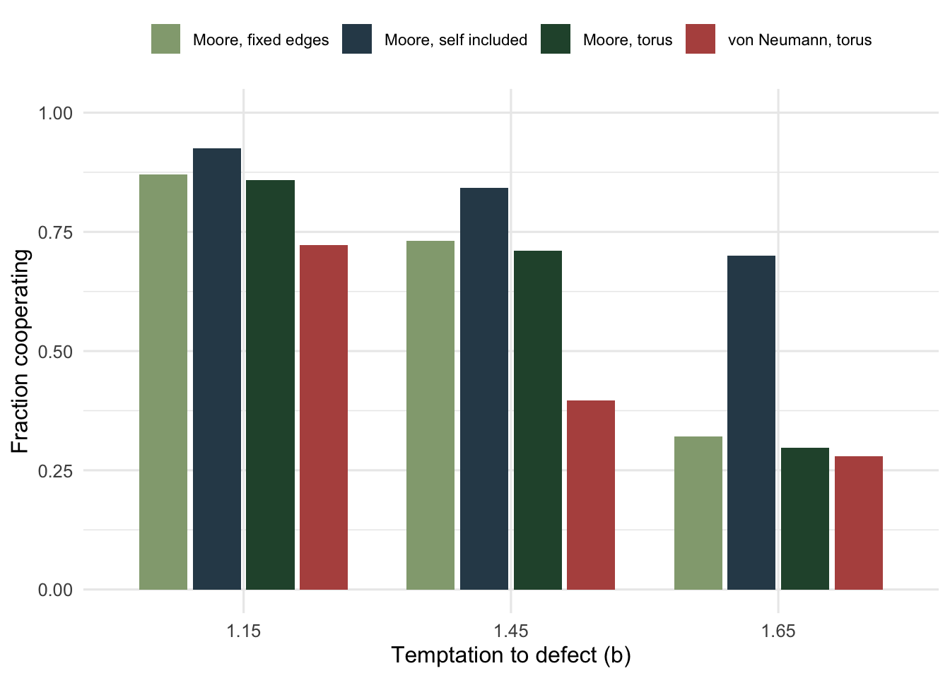
image-alt: "Grouped bars comparing cooperator frequency across four lattice model variants at three temptation levels, with the self-interaction variant highest everywhere but far above the rest only at the strongest temptation."
---
*Corrected 14 October 2026: the seed check compared this model with the reputation models using a spread across seeds that dated from before that post's own correction; it now says only that the spread there, under image scoring, was at least an order of magnitude larger.*
*Corrected 1 October 2026: the introduction said that one of the four modelling choices changes the answer enough to matter, and it now says that three do and only the starting seed does not; the snowdrift check said the four-neighbour lattice falls below the well-mixed mixture once the cost reaches half the benefit, and it now says it does so only at the two middle costs, since at the highest cost it sits above.*
The lattice model two posts back produced a clean result: cooperators hold about 0.71 of the lattice at a temptation of 1.45, and they die out in a well-mixed population with the same payoffs. That result rests on four choices that were never examined. Everything updated at once. The neighbourhood was the eight surrounding cells. The starting lattice came from one seed. And the game was a prisoner's dilemma.
Each of those has been the subject of a published objection, and three of the four change the answer enough to matter; only the starting seed does not. This post runs all four checks with one engine, so the variants differ only in the argument passed.
## One engine, four switches
The engine below takes any two-by-two payoff matrix, a neighbourhood list, and switches for the torus, self-interaction and asynchronous updating. Asynchronous updating cannot be vectorised across cells the way the synchronous rule can, so it keeps a running count of cooperating neighbours and repairs it after each flip. That turns an otherwise quadratic loop into a linear one.
```{r}
#| label: engine
nb_moore <- list(c(-1,-1), c(-1,0), c(-1,1), c(0,-1), c(0,1), c(1,-1), c(1,0), c(1,1))
nb_vn    <- list(c(-1,0), c(0,-1), c(0,1), c(1,0))

neighbours <- function(n, nb, torus = TRUE) {
  rr <- rep(seq_len(n), times = n); cc <- rep(seq_len(n), each = n)
  out <- matrix(NA_integer_, n * n, length(nb))
  for (j in seq_along(nb)) {
    r <- rr + nb[[j]][1]; c <- cc + nb[[j]][2]
    if (torus) {
      out[, j] <- ((c - 1) %% n) * n + ((r - 1) %% n) + 1
    } else {
      ok <- r >= 1 & r <= n & c >= 1 & c <= n
      out[ok, j] <- (c[ok] - 1) * n + r[ok]
    }
  }
  out
}

pay_of <- function(z, nC, deg, A, self) {
  if (self) { nC <- nC + z; deg <- deg + 1 }
  ifelse(z == 1, A[1,1] * nC + A[1,2] * (deg - nC),
                 A[2,1] * nC + A[2,2] * (deg - nC))
}

run_game <- function(n = 50, A, p0 = 0.9, gens = 150, seed = 1, nb = nb_moore,
                     torus = TRUE, self = FALSE, async = FALSE) {
  set.seed(seed)
  NI  <- neighbours(n, nb, torus)
  N   <- n * n
  deg <- rowSums(!is.na(NI))
  S   <- rbinom(N, 1, p0)
  count <- function(S) vapply(seq_len(N), function(i) {
    j <- NI[i, ]; sum(S[j[!is.na(j)]]) }, numeric(1))
  nC  <- count(S)
  fc  <- numeric(gens + 1); fc[1] <- mean(S)
  for (g in seq_len(gens)) {
    if (!async) {
      P    <- pay_of(S, nC, deg, A, self)
      cand <- cbind(P, matrix(P[NI], N, ncol(NI)))
      cs   <- cbind(S, matrix(S[NI], N, ncol(NI)))
      cand[is.na(cand)] <- -Inf
      S  <- cs[cbind(seq_len(N), max.col(cand, ties.method = "first"))]
      nC <- count(S)
    } else {
      for (i in sample.int(N)) {
        j   <- NI[i, ]; j <- j[!is.na(j)]
        set <- c(i, j)
        new <- S[set][which.max(pay_of(S[set], nC[set], deg[set], A, self))]
        if (new != S[i]) { nC[j] <- nC[j] + (new - S[i]); S[i] <- new }
      }
    }
    fc[g + 1] <- mean(S)
  }
  list(S = matrix(S, n, n), fc = fc)
}

pd        <- function(b) matrix(c(1, b, 0, 0), 2, 2)
snowdrift <- function(b, cost) matrix(c(b - cost/2, b, b - cost, 0), 2, 2)
xstar     <- function(M) (M[2,2] - M[1,2]) / (M[1,1] - M[1,2] - M[2,1] + M[2,2])
tail_mean <- function(r, k = 50) mean(tail(r$fc, k))

baseline_50 <- tail_mean(run_game(A = pd(1.45)))
cat("baseline, 50 by 50, temptation 1.45:", round(baseline_50, 4), "\n")
```
The baseline sits at `r sprintf("%.4f", baseline_50)` on this smaller lattice, against 0.71 on the 100 by 100 one. That is the first thing worth knowing: both numbers sit inside the seed to seed range measured in check 3 below, so lattice size does not move the story.
## Check 1: does everything have to move at once?
Synchronous updating means the whole lattice recomputes from the same snapshot. Huberman and Glance pointed out in 1993 that this is a strong assumption, that no real population does it, and that some of the striking patterns in the original model depend on it. Nowak, Bonhoeffer and May replied that the qualitative conclusion survives. Both claims can be tested directly, and one asynchronous generation is defined here as `N` single-cell updates in random order, so the two schemes do the same amount of work.
```{r}
#| label: async
for (b in c(1.15, 1.45, 1.65)) {
  s <- mean(sapply(1:3, function(sd) tail_mean(run_game(A = pd(b), seed = sd))))
  a <- mean(sapply(1:3, function(sd) tail_mean(run_game(A = pd(b), seed = sd, async = TRUE))))
  cat(sprintf("temptation %.2f   synchronous %.4f   asynchronous %.4f\n", b, s, a))
}
```
Both sides of that argument were partly right. At a temptation of 1.15 and 1.45 cooperation survives under either scheme, though asynchronous updating costs about 8 points at 1.15 and 2 points at 1.45. At 1.65 the schemes disagree completely: synchronous updating leaves cooperators at about 0.30 while asynchronous updating drives them to zero.
The honest summary is that the existence of the effect survives a change of update timing and the location of the collapse does not. So a paper reporting "cooperation persists in a spatial model" is on safe ground, and a paper reporting a critical temptation value from a synchronous lattice is reporting a property of the update scheme as much as of the game.
## Check 2: neighbourhood, edges, and one footnote that matters
Three conventions get chosen almost without comment when a lattice model is written. Whether the neighbourhood is the four orthogonal cells or all eight. Whether the lattice wraps or has real edges. And whether a player is counted as interacting with itself, which the 1992 paper did and most later work does not.
```{r}
#| label: fig-variants
#| fig-cap: "Cooperator frequency under four combinations of lattice conventions, at three values of the temptation. Averages of three seeds over the last 50 of 150 generations on a 50 by 50 lattice."
#| fig-alt: "Grouped bars at three temptation values, with the self-included variant highest everywhere and von Neumann lowest at the middle temptation."
library(ggplot2)
te_canvas <- theme(plot.background  = element_rect(fill = "#f5f4ee", colour = NA),
                   panel.background = element_rect(fill = "#f5f4ee", colour = NA))
variants <- list(
  `Moore, torus`         = list(nb = nb_moore, torus = TRUE,  self = FALSE),
  `von Neumann, torus`   = list(nb = nb_vn,    torus = TRUE,  self = FALSE),
  `Moore, fixed edges`   = list(nb = nb_moore, torus = FALSE, self = FALSE),
  `Moore, self included` = list(nb = nb_moore, torus = TRUE,  self = TRUE))

grid <- do.call(rbind, lapply(names(variants), function(nm) {
  v <- variants[[nm]]
  do.call(rbind, lapply(c(1.15, 1.45, 1.65), function(b) {
    fc <- mean(sapply(1:3, function(sd) tail_mean(
      run_game(A = pd(b), seed = sd, nb = v$nb, torus = v$torus, self = v$self))))
    data.frame(variant = nm, b = b, fc = fc)
  }))
}))
wide <- reshape(grid, idvar = "variant", timevar = "b", direction = "wide")
wide[-1] <- round(wide[-1], 4)
print(wide, row.names = FALSE)
ggplot(grid, aes(factor(b), fc, fill = variant)) +
  geom_col(position = position_dodge(width = 0.8), width = 0.72) +
  scale_fill_manual(values = c(`Moore, torus` = "#275139",
                               `von Neumann, torus` = "#b5534e",
                               `Moore, fixed edges` = "#93a87f",
                               `Moore, self included` = "#2f4858")) +
  ylim(0, 1) +
  labs(x = "Temptation to defect (b)", y = "Fraction cooperating", fill = NULL) +
  theme_minimal(base_size = 12) + te_canvas +
  theme(legend.position = "top", legend.text = element_text(size = 8.5))
```
Wrapping the lattice barely matters: fixed edges give slightly more cooperation, because corner and edge cells have fewer neighbours and small groups are easier for cooperators to hold. The neighbourhood matters a lot at intermediate temptation, where four neighbours give 0.40 against eight neighbours giving 0.71. Four-neighbour blocks have proportionally more boundary, and boundaries are where cooperators lose.
The largest effect comes from the convention that looks most like a footnote. Counting a player as one of its own partners lifts cooperation at every temptation, and at 1.65 it moves the result from 0.30 to 0.70. It does this because a cooperator's self-interaction pays 1 while a defector's pays 0, so the convention quietly hands every cooperator a bonus that no defector receives. Anyone comparing a modern lattice result with the 1992 numbers is comparing two different models, and the difference is larger than most of the effects being discussed.
## Check 3: is one seed enough?
The earlier post used a single starting lattice. Ten seeds show how much that mattered.
```{r}
#| label: seeds
for (b in c(1.45, 1.65)) {
  v <- sapply(1:10, function(sd) tail_mean(run_game(A = pd(b), seed = sd)))
  cat(sprintf("temptation %.2f   mean %.4f   sd %.4f   range %.4f to %.4f\n",
              b, mean(v), sd(v), min(v), max(v)))
}
```
Very little. The standard deviation across ten seeds is 0.0124 at a temptation of 1.45 and 0.0034 at 1.65, so a single run lands within a few percentage points of the ten-seed mean. This model is the well-behaved case: a large deterministic lattice averages over its own initial randomness, and reporting one run is defensible here in a way it was not for the agent-based reputation models, where the standard deviation across seeds under image scoring was at least an order of magnitude larger than either value here.
Cheap to check, and worth checking, because you cannot tell in advance which kind of model you have.
## Check 4: is it the space, or is it the game?
The most substantive objection to network reciprocity is that "space helps cooperation" is not a general result. Hauert and Doebeli made the case with the snowdrift game, where the cost of a shared job is split by whoever does it, and free-riding is tempting but doing the job alone still beats leaving it undone. Well-mixed, that game settles at a mixture instead of collapsing, so there is a non-trivial baseline to compare against.
```{r}
#| label: snow
for (cost in c(0.3, 0.5, 0.7, 0.9)) {
  A  <- snowdrift(1, cost)
  m8 <- mean(sapply(1:3, function(sd) tail_mean(run_game(A = A, seed = sd))))
  m4 <- mean(sapply(1:3, function(sd) tail_mean(run_game(A = A, seed = sd, nb = nb_vn))))
  cat(sprintf("cost %.1f   well-mixed %.4f   eight neighbours %.4f   four neighbours %.4f\n",
              cost, xstar(A), m8, m4))
}
```
With four neighbours the lattice sits below the well-mixed mixture at the two middle costs, and by a cost of 0.7 it is at 0.28 against a well-mixed 0.46. Spatial structure has made cooperation worse. With eight neighbours and the same cost it goes the other way, reaching 0.75 against that same 0.46. The ordering is not fixed across the cost range either: at a cost of 0.3 the four-neighbour lattice sits just above the mixture and the eight-neighbour one just below, and at 0.9 both sit above it.
So the sign of the spatial effect depends on the game, on the neighbourhood size and on the cost, in the same engine, with the same update rule and the same seeds. That is a stronger caution than any of the first three checks. It means a result of the form "structure promotes cooperation" is not transferable: it has to be re-derived for the payoff structure and the interaction geometry at hand.
The previous post reached the opposite conclusion for the snowdrift game from the Ohtsuki and Nowak transform, which predicted structure pushing the mixture up at every degree. Both are correct within their assumptions. The transform describes weak selection with death-birth replacement; this lattice runs strong selection with deterministic imitation. They are answers to different questions that happen to share a vocabulary, and conflating them is easy to do by accident.
## An honest limit
These are internal checks. They tell you which of the model's conclusions are artefacts of its own settings, and nothing at all about whether the model applies to any organism. The four choices examined here are also not exhaustive: mutation, mobility, continuous space, heterogeneous degree and payoff noise are all absent, and each of them has its own literature.
The deeper problem is that the model has no independent way to fix its own parameters. A temptation of 1.45 was chosen because it sits inside the interesting range, not because anything was measured. Until the payoffs come from an experiment, a lattice model is a device for working out what follows from a set of assumptions, which is a real use, but not the same as evidence about a population.
## References
Huberman BA, Glance NS 1993. Proceedings of the National Academy of Sciences 90(16):7716-7718 (10.1073/pnas.90.16.7716)
Nowak MA, Bonhoeffer S, May RM 1994. Proceedings of the National Academy of Sciences 91(11):4877-4881 (10.1073/pnas.91.11.4877)
Hauert C, Doebeli M 2004. Nature 428(6983):643-646 (10.1038/nature02360)
Ohtsuki H, Hauert C, Lieberman E, Nowak MA 2006. Nature 441(7092):502-505 (10.1038/nature04605)
## Related tutorials
- [Network reciprocity on a lattice](../network-reciprocity-on-a-lattice/)
- [Update rules and cooperation on graphs](../update-rules-and-cooperation/)
- [Checking a reciprocity model](../checking-a-reciprocity-model/)
- [Checking a game theory model](../checking-a-game-theory-model/)