shift <- function(M, dr, dc) {
  n <- nrow(M); m <- ncol(M)
  M[((seq_len(n) - 1 + dr) %% n) + 1, ((seq_len(m) - 1 + dc) %% m) + 1, drop = FALSE]
}

nb8 <- list(c(-1,-1), c(-1,0), c(-1,1), c(0,-1), c(0,1), c(1,-1), c(1,0), c(1,1))

payoff_field <- function(S, b) {
  nC <- Reduce(`+`, lapply(nb8, function(d) shift(S, d[1], d[2])))
  ifelse(S == 1, nC, b * nC)          # 1 = cooperator, 0 = defector
}

step_lattice <- function(S, b) {
  P <- payoff_field(S, b)
  best <- P; winner <- S
  for (d in nb8) {
    Pn <- shift(P, d[1], d[2]); Sn <- shift(S, d[1], d[2])
    take <- Pn > best
    best[take] <- Pn[take]
    winner[take] <- Sn[take]
  }
  winner
}

run_lattice <- function(n = 100, b = 1.45, p0 = 0.9, gens = 200, seed = 1) {
  set.seed(seed)
  S <- matrix(rbinom(n * n, 1, p0), n, n)
  fc <- numeric(gens + 1); fc[1] <- mean(S)
  for (g in seq_len(gens)) {
    S <- step_lattice(S, b)
    fc[g + 1] <- mean(S)
  }
  list(S = S, fc = fc)
}Network reciprocity on a lattice
evolutionary ecology
evolutionary game theory
spatial ecology
R
ecology tutorial
Simulate the spatial prisoner’s dilemma in base R: cooperator clusters survive on a lattice at benefit-to-cost ratios where a well-mixed population loses them.
Corrected 30 September 2026: the well-mixed comparison was described as having each player play actual random partners; it now says that each player receives the payoff it would expect from random partners, which is what the code computes.
In a well-mixed prisoner’s dilemma defection dominates: whatever the other player does, defecting pays more. That result assumes every player is equally likely to meet every other player, which is close to false for anything rooted, sessile, territorial or philopatric. Plants compete with the plants beside them. Ant colonies interact with the colonies whose foraging ranges overlap theirs. A soil bacterium’s siderophores diffuse a few hundred micrometres.
Relax the mixing assumption and cooperation can survive without memory, without recognition, and without reputation. Cooperators that happen to sit next to each other collect benefits from each other, and a cluster of them can hold ground against defectors that would win every isolated contest. That is network reciprocity, and it is the cheapest of the routes to cooperation in the sense that it requires nothing of the organism at all: only that interaction is local.
This post builds the model that made the point, from Nowak and May’s 1992 lattice, in base R.
The model
Each cell of a square lattice holds a cooperator or a defector. Every player plays a one-shot prisoner’s dilemma with each of its eight surrounding neighbours and adds up the payoffs. Then every player looks at itself and its eight neighbours and adopts the strategy of whoever scored highest.
The payoffs use the weak form of the dilemma: cooperating against a cooperator pays 1, cooperating against a defector pays 0, defecting against a cooperator pays b > 1, and mutual defection pays 0. Setting the two lowest payoffs equal removes one free parameter and leaves b as the only thing to vary. It also makes the dilemma slightly less severe than the general case, which is worth remembering when the results look encouraging.
The lattice wraps around at the edges, so it is a torus and no cell is special. Everything below is written with matrix shifts rather than loops, which keeps a 100 by 100 lattice fast enough to sweep parameters.
A defector’s payoff is b times its number of cooperating neighbours, and a cooperator’s payoff is one times the same count. Neither strategy earns anything from a defecting neighbour, which is what the weak dilemma buys.
Cooperators persist
Start from a lattice that is 90 per cent cooperators and let it run at b = 1.45.
r <- run_lattice(b = 1.45)
cat(sprintf("start %.4f   generation 10 %.4f   generation 50 %.4f   final %.4f\n",
            r$fc[1], r$fc[11], r$fc[51], r$fc[201]))
start 0.8956 generation 10 0.6788 generation 50 0.7037 final 0.7066cat(sprintf("last 50 generations: mean %.4f, sd %.4f\n",
mean(r$fc[152:201]), sd(r$fc[152:201])))last 50 generations: mean 0.7092, sd 0.0025Cooperators drop sharply at the start, as the defectors scattered through the initial lattice each eat into their surroundings, and then the decline reverses. Cooperator frequency bottoms out at 0.3562 in the second generation and climbs back as the surviving cooperator blocks grow into the space the defectors cleared. The population settles near 0.71 and stays there, fluctuating by a few parts in a thousand.
library(ggplot2)
te_canvas <- theme(plot.background  = element_rect(fill = "#f5f4ee", colour = NA),
                   panel.background = element_rect(fill = "#f5f4ee", colour = NA))
ggplot(data.frame(g = 0:200, fc = r$fc), aes(g, fc)) +
  geom_hline(yintercept = 0, colour = "#8d8d80") +
  geom_line(colour = "#275139", linewidth = 0.9) +
  ylim(0, 1) +
  labs(x = "Generation", y = "Fraction cooperating") +
  theme_minimal(base_size = 12) + te_canvas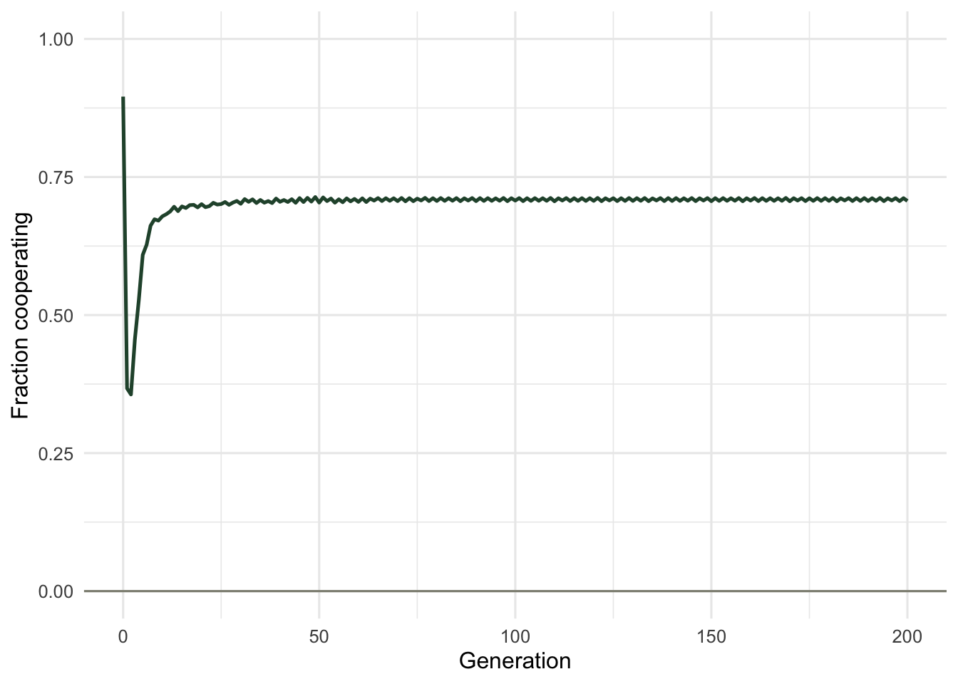
The plateau is not an equilibrium in the usual sense. Individual cells keep switching; the boundaries between cooperator patches and defector patches keep moving. What is stable is the statistical composition, and that is a different claim from a fixed point.
Where the stability comes from
The lattice snapshot shows why. Cooperators are not spread evenly through the survivors; they sit in solid blocks.
grid <- expand.grid(row = 1:100, col = 1:100)
grid$strategy <- factor(ifelse(as.vector(r$S) == 1, "cooperate", "defect"))
ggplot(grid, aes(col, row, fill = strategy)) +
  geom_raster() +
  scale_fill_manual(values = c(cooperate = "#275139", defect = "#b5534e")) +
  coord_equal() +
  labs(x = NULL, y = NULL, fill = NULL) +
  theme_void(base_size = 12) + te_canvas + theme(legend.position = "top")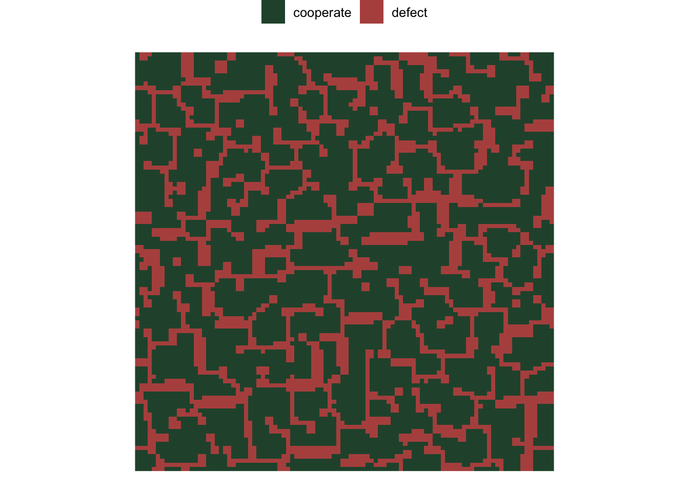
Clustering can be measured rather than eyeballed. Count, for every cell, how many of its eight neighbours share its strategy, and compare that with a lattice reshuffled to the same overall frequency.
concordance <- function(S) {
  same <- Reduce(`+`, lapply(nb8, function(d) as.numeric(shift(S, d[1], d[2]) == S)))
  mean(same) / 8
}
set.seed(1)
reshuffled <- matrix(rbinom(10000, 1, mean(r$S)), 100, 100)
cat(sprintf("neighbour concordance: simulated %.4f, reshuffled %.4f\n",
            concordance(r$S), concordance(reshuffled)))
neighbour concordance: simulated 0.7519, reshuffled 0.5828Three quarters of neighbour pairs share a strategy in the simulated lattice, against 0.58 in a random lattice with the same cooperator frequency. The spatial correlation is the mechanism. A defector on a straight block edge touches three cooperators and earns 3b, or 4.35 at this benefit, against the 5 earned by the edge cooperator beside it, so the defector copies the cooperator and the block advances. That holds while 3b is below 5, that is while b is below 5/3, which is where the sweep below puts the collapse. Defectors survive in the gaps, where the geometry runs the other way: one wedged in a single-cell channel between two blocks touches six cooperators and earns 8.7, more than any cooperator on the lattice can earn.
How far it goes
The interesting question is how large b can get before clustering stops being enough. Sweep it, with three initial lattices per value.
bs <- seq(1.05, 2.00, by = 0.05)
sweep <- do.call(rbind, lapply(bs, function(b) {
  v <- sapply(1:3, function(s)
    mean(run_lattice(n = 80, b = b, gens = 200, seed = s)$fc[152:201]))
  data.frame(b = b, mean = mean(v), lo = min(v), hi = max(v))
}))
print(round(sweep, 4), row.names = FALSE)
b mean lo hi
1.05 0.9161 0.9154 0.9170
1.10 0.9161 0.9154 0.9170
1.15 0.8597 0.8566 0.8630
1.20 0.8449 0.8385 0.8535
1.25 0.8208 0.8084 0.8296
1.30 0.8153 0.8050 0.8227
1.35 0.7901 0.7763 0.8075
1.40 0.7084 0.7041 0.7136
1.45 0.7084 0.7041 0.7136
1.50 0.7709 0.7666 0.7749
1.55 0.7422 0.7369 0.7450
1.60 0.4145 0.4085 0.4183
1.65 0.2988 0.2969 0.2999
1.70 0.0658 0.0527 0.0784
1.75 0.0421 0.0362 0.0497
1.80 0.0366 0.0302 0.0422
1.85 0.0366 0.0302 0.0422
1.90 0.0366 0.0302 0.0422
1.95 0.0366 0.0302 0.0422
2.00 0.0159 0.0111 0.0219ggplot(sweep, aes(b, mean)) +
geom_ribbon(aes(ymin = lo, ymax = hi), fill = "#93a87f", alpha = 0.45) +
geom_line(colour = "#275139", linewidth = 0.8) +
geom_point(colour = "#275139", size = 1.6) +
ylim(0, 1) +
labs(x = "Benefit of defecting (b)", y = "Fraction cooperating") +
theme_minimal(base_size = 12) + te_canvas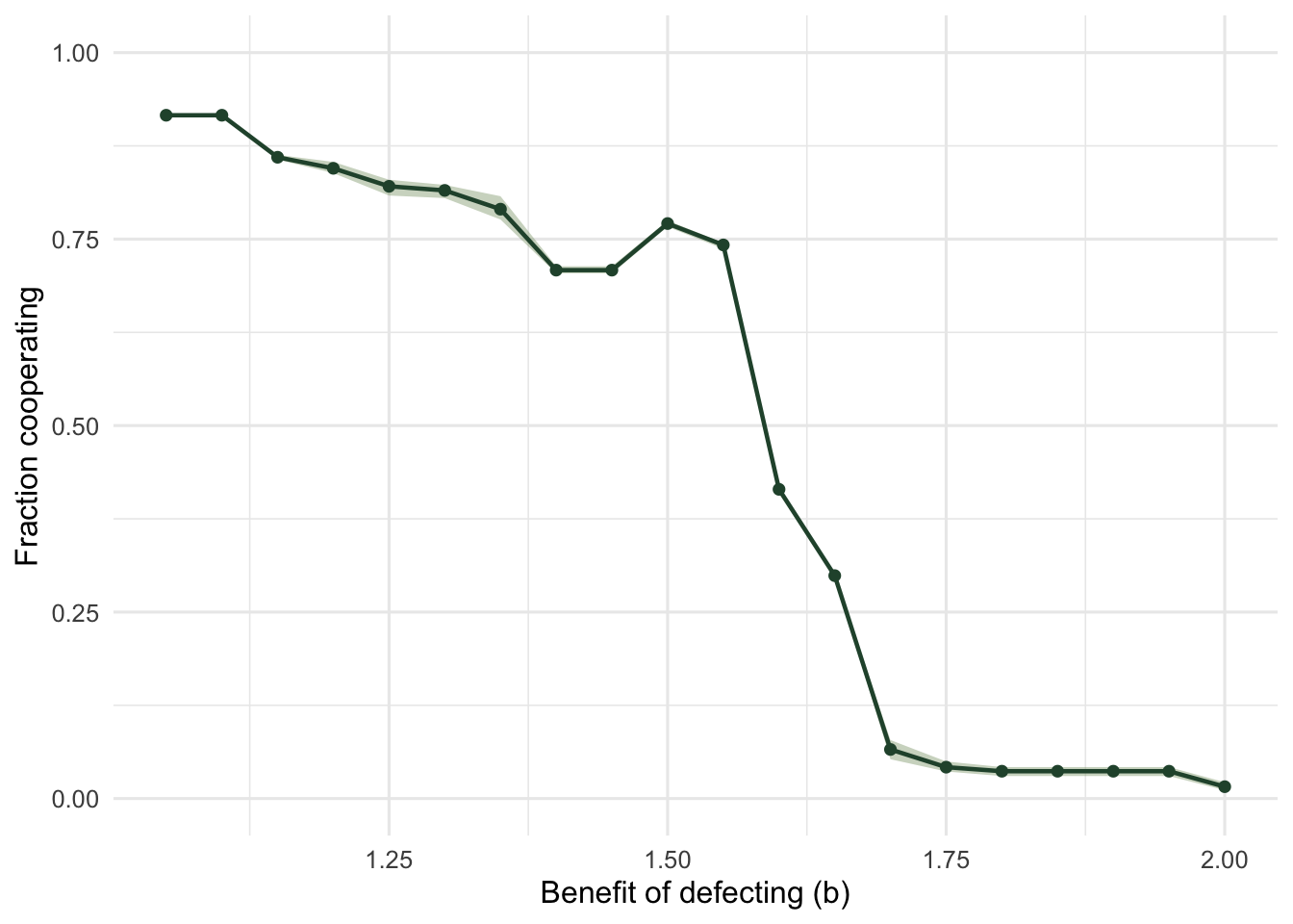
Cooperation holds above 0.70 all the way to b = 1.55, drops to 0.4145 at 1.60, and is down to 0.0658 by 1.70: reduced to a few isolated pockets rather than extinct. The three seeds barely separate, so the outcome is a property of b rather than of the starting lattice.
The shape of that curve is worth a second look, because it is not a curve. It is a staircase with flat treads: 1.05 and 1.10 give the same answer to four decimals, so do 1.40 and 1.45, and so do 1.80 through 1.95. It is not even monotone. The value at 1.50 (0.7709) sits above the value at 1.45 (0.7084), because a change in which payoff comparisons tie can reorganise the geometry of the blocks in a way that happens to favour cooperators slightly. The reason is that an imitate-the-best rule only ever compares payoffs, and with these integer-weighted payoffs the comparisons only flip when b crosses a ratio of small whole numbers. Between those crossings nothing changes. Reporting a smooth relationship between benefit and cooperation from this model would be reading structure into it that is not there, and the treads also mean a fitted threshold is only ever accurate to the width of a tread.
The comparison that matters
None of this is impressive on its own. It becomes a result only against the well-mixed case, so remove the space and keep everything else. Every player still copies the best of nine, with role models now drawn at random from the whole population, but instead of playing eight actual partners each player receives the payoff it would expect from eight random ones: eight times the cooperator frequency, multiplied by b for a defector.
Without space, every cooperator has the same expected payoff and so does every defector, and the defector’s is larger whenever any cooperator exists. So a player keeps cooperating only if all eight of its role models happen to be cooperators, which happens with probability x^8, and it must itself be a cooperator, giving x' = x^9.
sim_wellmixed <- function(N = 10000, b = 1.45, p0 = 0.9, gens = 6, seed = 1) {
  set.seed(seed)
  S <- rbinom(N, 1, p0)
  x <- numeric(gens + 1); x[1] <- mean(S)
  for (g in seq_len(gens)) {
    xx <- mean(S)
    P <- ifelse(S == 1, 8 * xx, b * 8 * xx)
    mod <- matrix(sample.int(N, N * 8, replace = TRUE), N, 8)
    cand <- cbind(P, matrix(P[mod], N, 8))
    cs   <- cbind(S, matrix(S[mod], N, 8))
    S <- cs[cbind(seq_len(N), max.col(cand, ties.method = "first"))]
    x[g + 1] <- mean(S)
  }
  x
}
sim <- sim_wellmixed()
pred <- numeric(length(sim)); pred[1] <- sim[1]
for (g in seq_len(length(sim) - 1)) pred[g + 1] <- pred[g]^9
cat("simulated:", format(round(sim, 6), scientific = FALSE), "\n")
simulated: 0.8956 0.3663 0.0000 0.0000 0.0000 0.0000 0.0000 cat("x^9 rule :", format(round(pred, 6), scientific = FALSE), "\n")x^9 rule : 0.895600 0.370704 0.000132 0.000000 0.000000 0.000000 0.000000 cat("largest discrepancy:", format(max(abs(sim - pred)), digits = 3), "\n")largest discrepancy: 0.0044 Cooperators are extinct by generation three. The same players, the same payoffs and the same imitation rule give 0.71 on a lattice and 0 in a well-mixed population. The x^9 recursion tracks the simulation to within 0.005, which is a useful sanity check: when a simple analytic prediction and a simulation agree, both are probably implemented correctly.
An honest limit
The result is real but the model is severe. Updating is synchronous, so the whole lattice steps at once; imitation is deterministic best-takes-all, with no error and no noise; the neighbourhood is fixed at eight; and the weak dilemma sets two of the four payoffs equal. Each of those is a choice, and Huberman and Glance showed as early as 1993 that the synchrony in particular does real work, with Nowak, Bonhoeffer and May replying that the qualitative conclusion survives asynchronous updating. Two later posts take those objections seriously: one replaces the simulation with an exact calculation for general graphs, and one runs the diagnostics.
There is also a limit that no amount of checking removes. This model says that local interaction can maintain cooperation, not that it does maintain any particular case of cooperation in the field. Demonstrating network reciprocity in a real population means showing that interaction really is local at the relevant scale, that the payoffs really have this structure, and that relatedness is not doing the work instead. Spatial clustering generates relatedness as a side effect, so a lattice model and a kin selection model are not competing explanations here; they are two descriptions of the same clustering.
References
Nowak MA, May RM 1992. Nature 359(6398):826-829 (10.1038/359826a0)
Huberman BA, Glance NS 1993. Proceedings of the National Academy of Sciences 90(16):7716-7718 (10.1073/pnas.90.16.7716)
Nowak MA, Bonhoeffer S, May RM 1994. Proceedings of the National Academy of Sciences 91(11):4877-4881 (10.1073/pnas.91.11.4877)
Nowak MA 2006. Science 314(5805):1560-1563 (10.1126/science.1133755)