on_transform <- function(A, k, nu) {
  D   <- matrix(diag(A), ncol = 1)
  one <- matrix(1, nrow(A), 1)
  A + (D %*% t(one) - one %*% t(D)) / (k - 2) + nu * (A - t(A)) / (k - 2)
}

nu_of <- function(rule, k) switch(rule, BD = 1, DB = 1 / (k + 1), IM = 3 / (k + 3))Update rules and cooperation on graphs
evolutionary ecology
evolutionary game theory
spatial ecology
R
ecology tutorial
Implement the Ohtsuki and Nowak transform in R and recover the b/c > k rule: whether spatial structure favours cooperation depends on the replacement rule.
Corrected 8 October 2026: the snowdrift section said without qualification that the mixture of cooperators and defectors survives on the graph; it now limits that to the cost and the degrees in the loop, and says that a smaller neighbourhood or a cheaper job can let cooperation dominate outright.
Corrected 1 October 2026: the post credited the transformed payoff matrix to the four-author Nature paper, which gives the b/c > k rule but not the transform; the post no longer credits that paper with it, and the explanation of why death-birth updating favours cooperation now says that a cooperator’s help and its competition for a vacancy fall largely on different individuals. The limitations section no longer says that loops make the b/c > k rule itself an approximation on a large lattice.
Corrected 27 September 2026: the text alternative for the threshold figure described a shaded region favouring defection that the figure does not draw; it now describes only the two lines.
The lattice simulation in the previous post answers a question about one specific model: a torus, eight neighbours, synchronous steps, deterministic copy-the-best. Change any of those and the numbers change. What we would rather have is a statement about graphs in general, and there is one.
Under weak selection, a game played on a regular graph of degree k behaves like a different game played in a well-mixed population: exactly so in the limit of large graphs without short loops, and closely enough to be useful otherwise. The graph does not need its own theory. It gets absorbed into a modified payoff matrix, and everything already known about well-mixed two-strategy games then applies. The modification depends on k and on one number that encodes how individuals are replaced.
That last part is the interesting one, because it turns out the replacement rule is not a technical detail. It decides whether spatial structure helps cooperation at all.
Three ways to update a population
All three rules keep the population size fixed and use payoff to set reproductive success. They differ in who competes with whom.
Under birth-death, one individual is chosen to reproduce with probability proportional to fitness, anywhere in the graph, and its offspring replaces a random neighbour. Competition to reproduce is global; only the death is local.
Under death-birth, one individual is chosen to die at random, and its neighbours compete to fill the gap in proportion to fitness. Competition is local on the reproduction side.
Under imitation, one individual is chosen at random and then either keeps its own strategy or copies a neighbour, with the choice weighted by fitness. It is death-birth with the focal individual added to the competition.
The transform
Write A for the payoff matrix, Delta for its diagonal as a column vector, and 1 for a column of ones. The graph-adjusted matrix is
\[B = A + \frac{1}{k-2}\left(\Delta \mathbf{1}^{\mathsf T} - \mathbf{1}\Delta^{\mathsf T}\right) + \frac{\nu}{k-2}\left(A - A^{\mathsf T}\right)\]
with nu = 1 for birth-death, 1/(k+1) for death-birth and 3/(k+3) for imitation. It fits in five lines of base R.
The two correction terms are both antisymmetric, so they add nothing along the diagonal: a strategy’s payoff against itself is untouched. What the graph changes is how strategies fare against each other, which is exactly where a dilemma lives.
Two things to note before using it. The denominator k - 2 means the transform says nothing about k = 2, a cycle, and nothing about k = 1. And weak selection is a real restriction, not decoration: payoff differences must be small relative to baseline fitness. The result is a statement about the direction of a small bias, not about a population where cooperating doubles your offspring count.
The donation game
The cleanest cooperation payoff structure is the donation game. A cooperator pays a cost c to give a benefit b to its partner; a defector pays nothing and gives nothing. Over the strategy order (C, D) that is a matrix with b - c for mutual cooperation, -c for cooperating against a defector, b for exploiting a cooperator, and 0 for mutual defection.
donation <- function(b, cost) {
  matrix(c(b - cost, b, -cost, 0), 2, 2, dimnames = list(c("C", "D"), c("C", "D")))
}

classify <- function(B) {
  d1 <- B["C", "C"] - B["D", "C"]      # C minus D against a cooperator
  d2 <- B["C", "D"] - B["D", "D"]      # C minus D against a defector
  if (d1 > 0 && d2 > 0)      "C dominates"
  else if (d1 < 0 && d2 < 0) "D dominates"
  else if (d1 > 0 && d2 < 0) "bistable"
  else                       "coexistence"
}

print(donation(5, 1))
C D
C 4 -1
D 5 0print(round(on_transform(donation(5, 1), k = 4, nu = nu_of("DB", 4)), 4)) C D
C 4.0 0.4
D 3.6 0.0The original matrix is a prisoner’s dilemma: 5 beats 4 in the first column, 0 beats -1 in the second, so defection dominates. The transformed matrix has cooperation earning 4 against a cooperator where defection earns 3.6, and 0.4 against a defector where defection earns 0. Cooperation now dominates. Nothing about the players changed; only the accounting for who they compete with.
The thresholds
Sweep the benefit at fixed cost and find where each rule flips, by bisection rather than by algebra.
threshold <- function(rule, k, hi = 1e4) {
  favoured <- function(b)
    classify(on_transform(donation(b, 1), k, nu_of(rule, k))) == "C dominates"
  if (!favoured(hi)) return(NA_real_)
  lo <- 1
  for (i in 1:200) { mid <- (lo + hi) / 2; if (favoured(mid)) hi <- mid else lo <- mid }
  (lo + hi) / 2
}

ks  <- c(3, 4, 5, 6, 8, 10, 16, 20, 50)
tab <- data.frame(k = ks,
                  BD = sapply(ks, threshold, rule = "BD"),
                  DB = sapply(ks, threshold, rule = "DB"),
                  IM = sapply(ks, threshold, rule = "IM"))
print(tab, row.names = FALSE)
k BD DB IM
3 NA 3 5
4 NA 4 6
5 NA 5 7
6 NA 6 8
8 NA 8 10
10 NA 10 12
16 NA 16 18
20 NA 20 22
50 NA 50 52cat("death-birth threshold equals k: ", all.equal(tab$DB, as.numeric(tab$k)), "\n")death-birth threshold equals k: TRUE cat("imitation threshold equals k + 2: ", all.equal(tab$IM, as.numeric(tab$k) + 2), "\n")imitation threshold equals k + 2: TRUE cat("birth-death has no threshold at all: ", all(is.na(tab$BD)), "\n")birth-death has no threshold at all: TRUE Three results, and the third is the one to keep.
Under death-birth updating, cooperation is favoured when b/c > k. This is the compact rule the 2006 Nature paper of Ohtsuki, Hauert, Lieberman and Nowak is known for, and the numerical search reproduces it to machine precision without any algebra being trusted. Under imitation the requirement is b/c > k + 2, harder by a constant. Under birth-death there is no benefit large enough. Spatial structure does not favour cooperation at all when reproduction competes globally.
library(ggplot2)
te_canvas <- theme(plot.background  = element_rect(fill = "#f5f4ee", colour = NA),
                   panel.background = element_rect(fill = "#f5f4ee", colour = NA))
d <- data.frame(k = rep(3:20, 2),
                thr = c(3:20, (3:20) + 2),
                rule = rep(c("death-birth", "imitation"), each = 18))
ggplot(d, aes(k, thr, colour = rule)) +
  geom_line(linewidth = 1) +
  geom_point(size = 1.5) +
  scale_colour_manual(values = c(`death-birth` = "#275139", imitation = "#b5534e")) +
  labs(x = "Neighbourhood size (k)", y = "Benefit-to-cost ratio needed",
       colour = NULL) +
  theme_minimal(base_size = 12) + te_canvas + theme(legend.position = "top")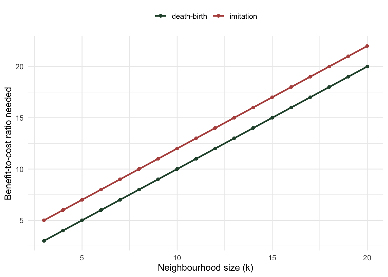
The practical reading is that the benefit of structure shrinks as neighbourhoods grow. At k = 4 a cooperative act needs to be four times more valuable to the recipient than it costs the actor, which is unremarkable for many plausible interactions. At k = 50 it needs to be fifty times more valuable, which is a strong demand. A well-mixed population is the limit k to infinity, and the threshold goes to infinity with it, which is the well-mixed result recovered from the other direction.
Why does the rule matter so much? Under death-birth, a cooperator competes for a vacancy only with the other neighbours of the individual that died, who are not its own neighbours unless the graph has triangles, while its help goes to its own neighbours, so the help and the competition fall largely on different individuals. Under birth-death, a cooperator’s success in the global reproduction lottery is paid for by the death of one of its own neighbours, and those neighbours are the ones who received its benefits. The help and the harm land on the same individuals and cancel. Local competition eating the benefit of local cooperation is the same problem that shows up in kin selection.
The same tool on a different game
Nothing about the transform assumes a dilemma. Apply it to the snowdrift game, where two players share the cost of a job that either would rather do alone than not have done: mutual cooperation pays b - c/2, cooperating alone pays b - c, free-riding on a cooperator pays b, and mutual defection pays nothing. Well-mixed, that game has a stable mixture rather than a winner.
snowdrift <- function(b, cost) {
  matrix(c(b - cost/2, b, b - cost, 0), 2, 2, dimnames = list(c("C","D"), c("C","D")))
}
xstar <- function(M) {
  (M["D","D"] - M["C","D"]) / (M["C","C"] - M["C","D"] - M["D","C"] + M["D","D"])
}

A <- snowdrift(b = 1, cost = 0.6)
cat(sprintf("well-mixed equilibrium: %.4f\n", xstar(A)))
well-mixed equilibrium: 0.5714for (k in c(4, 6, 8, 12, 20, 50, 200)) {
B <- on_transform(A, k, nu_of("DB", k))
cat(sprintf("k = %3d %-12s equilibrium %.4f\n", k, classify(B), xstar(B)))
}k = 4 coexistence equilibrium 0.9857
k = 6 coexistence equilibrium 0.7908
k = 8 coexistence equilibrium 0.7222
k = 12 coexistence equilibrium 0.6648
k = 20 coexistence equilibrium 0.6247
k = 50 coexistence equilibrium 0.5919
k = 200 coexistence equilibrium 0.5765For this cost and the degrees in the loop, the mixture survives and the graph only moves it; with a smaller neighbourhood or a cheaper job the transformed game can tip into one in which cooperation dominates outright. Under death-birth updating with a small neighbourhood the equilibrium is pushed strongly towards cooperation, and it slides back towards the well-mixed value of 0.5714 as the neighbourhood grows, reaching 0.5765 at k = 200. That convergence is a useful check on the implementation: a transform that did not recover the well-mixed game in the large-degree limit would be wrong somewhere.
An honest limit
Two restrictions do most of the damage. The first is weak selection, without which the transform does not hold at all; strong selection is a different regime and the results there need not agree. The second is the pair approximation behind the derivation, which assumes correlations between neighbours are captured by pair frequencies alone. On a real lattice, triangles and longer loops break that, so the transformed game is an approximation there. The approximation becomes exact in the limit of large graphs without short loops, and large random regular graphs come close to that. The b/c > k rule itself fares better than its derivation: for death-birth updating on a lattice with loops, the exact threshold approaches k as the lattice grows.
The snowdrift result above is a good illustration of how far that caution should go. It says structure raises cooperation under weak selection with death-birth updating. Hauert and Doebeli reported the opposite direction for the snowdrift game on lattices with strong-selection imitation dynamics, and both can be right, because they are statements about different regimes. The next post runs that comparison directly and finds that even the sign of the effect depends on the neighbourhood used.
Finally, the previous post’s lattice used the temptation parameterisation of a weak dilemma, not a benefit and a cost, so its collapse near a temptation of 1.6 is not comparable to a b/c threshold of 8. Two spatial models can both be correct and still refuse to be plotted on the same axis.
References
Ohtsuki H, Hauert C, Lieberman E, Nowak MA 2006. Nature 441(7092):502-505 (10.1038/nature04605)
Lieberman E, Hauert C, Nowak MA 2005. Nature 433(7023):312-316 (10.1038/nature03204)
Hauert C, Doebeli M 2004. Nature 428(6983):643-646 (10.1038/nature02360)
Nowak MA 2006. Science 314(5805):1560-1563 (10.1126/science.1133755)