make_pop <- function(p, r, G, n) {
  s <- sqrt(r); founder <- rbinom(G, 1, p)
  g <- as.vector(sapply(founder, function(f) ifelse(runif(n) < s, f, rbinom(n, 1, p))))
  list(g = g, grp = rep(seq_len(G), each = n))
}
sel_diff <- function(g, w) mean((w - mean(w)) * (g - mean(g))) / mean(w)Checking a kin selection analysis
evolutionary ecology
social evolution
model diagnostics
R
ecology tutorial
Three ways Hamilton’s rule misleads in R: non-additive payoffs, the scale of competition among relatives, and benefits that never reach any kin at all.
Corrected 7 October 2026: Check two said that under local competition a shared benefit lifts nobody’s relative fitness and that relatedness guarantees an altruist is subsidising its rivals; it now says that in the post’s model the benefit raises the recipients’ share of the group’s fixed output at the giver’s expense, so a larger benefit makes selection more negative and relatedness only softens the loss, and that the exact cancellation of benefit and competition belongs to other models of viscous populations.
Hamilton’s rule, rb > c, is the right first question about any cooperative behaviour, and a treacherous last answer. Its clean form hides three assumptions that field situations break routinely: that payoffs add up, that helped relatives are not also competitors, and that the benefit reaches kin in the first place. This post breaks each one in base R and watches the rule give the wrong prediction.
Check 1: payoffs must be additive
Hamilton’s rule is exact when the cost and benefit simply add. Real cooperation is often synergistic: helping pays off far more when a partner helps too. Add a synergy term and the additive threshold is wrong. Here relatedness is 0.5 and cost is 1, so rb > c says a benefit of 1.8 is not enough (rb - c = -0.1).
kin_sel <- function(b, c = 1, r = 0.5, p = 0.3, G = 12000, n = 4, syn = 0, seed = 2) {
  set.seed(seed); po <- make_pop(p, r, G, n); g <- po$g; grp <- po$grp
  g_oth <- (ave(g, grp, FUN = sum) - g) / (n - 1)
  sel_diff(g, 1 - c * g + b * g_oth + syn * g * g_oth)
}
cat(sprintf("additive,   b = 1.8 (rb - c = -0.10): selection = %+.4f\n", kin_sel(1.8, syn = 0)))
additive, b = 1.8 (rb - c = -0.10): selection = -0.0194cat(sprintf("synergistic, b = 1.8, syn = 2.0: selection = %+.4f\n", kin_sel(1.8, syn = 2.0)))synergistic, b = 1.8, syn = 2.0: selection = +0.1523The additive model behaves: selection is negative (-0.019), altruism does not spread, just as rb < c predicts. Add synergy and selection turns positive (+0.152): the allele spreads at a benefit where Hamilton’s rule said it should not. With non-additive payoffs the rule still works, but only if b is redefined as an average effect that already absorbs the synergy, which means the naive plug-in numbers mislead.
library(ggplot2)
te_canvas <- theme(plot.background  = element_rect(fill = "#f5f4ee", colour = NA),
                   panel.background = element_rect(fill = "#f5f4ee", colour = NA))
bs <- seq(0.5, 3, 0.25)
dd <- rbind(data.frame(b = bs, sel = vapply(bs, function(b) kin_sel(b, syn = 0), numeric(1)), payoff = "additive"),
            data.frame(b = bs, sel = vapply(bs, function(b) kin_sel(b, syn = 2.0), numeric(1)), payoff = "synergistic"))
ggplot(dd, aes(b, sel, colour = payoff)) +
  geom_hline(yintercept = 0, colour = "#93a87f", linewidth = 0.4) +
  geom_vline(xintercept = 2, linetype = "dashed", colour = "#93a87f") +
  geom_line(linewidth = 0.9) +
  scale_colour_manual(values = c(additive = "#275139", synergistic = "#b5534e")) +
  labs(x = "Benefit b", y = "Selection on allele", colour = NULL) +
  theme_minimal(base_size = 12) + te_canvas + theme(legend.position = "top")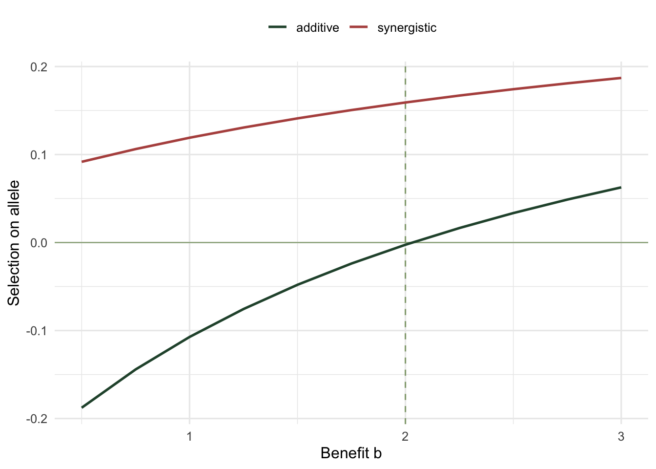
Check 2: the scale of competition
Helping a relative is worthless if that relative is also who you compete against. When competition is local, a benefit shared within the group lifts absolute fitness but not the group’s share of the population, and the altruism gains nothing (West and colleagues 2002; Queller 1994) or, in the model below, less than nothing. Compare global competition, where fitness is judged against the whole population, with fully local competition, where it is judged within the group.
kin_comp <- function(b, c = 1, r = 0.5, p = 0.3, a = 1, G = 12000, n = 4, seed = 4) {
  set.seed(seed); po <- make_pop(p, r, G, n); g <- po$g; grp <- po$grp
  g_oth <- (ave(g, grp, FUN = sum) - g) / (n - 1)
  w_abs <- 1 - c * g + b * g_oth
  sel_diff(g, w_abs - a * (ave(w_abs, grp, FUN = mean) - 1))   # a = local competition intensity
}
cat(sprintf("global competition (a = 0), b = 2.5 (rb - c = +0.25): selection = %+.4f\n", kin_comp(2.5, a = 0)))
global competition (a = 0), b = 2.5 (rb - c = +0.25): selection = +0.0374cat(sprintf("full local competition (a = 1), b = 2.5: selection = %+.4f\n", kin_comp(2.5, a = 1)))full local competition (a = 1), b = 2.5: selection = -0.1431Under global competition the allele spreads (+0.037), as rb > c promises. Under full local competition selection flips hard negative (-0.143): every unit of benefit an altruist hands to its group-mates raises their share of the group’s fixed output at its own expense. In this model a larger benefit therefore makes selection more negative, and relatedness only softens the loss. In other models of a viscous population, higher relatedness raises both the benefit of helping kin and the cost of competing with them, and the two can cancel exactly. Relatedness alone does not predict altruism; the scale of competition does half the work.
Check 3: the benefit has to reach kin
The rule assumes help lands on relatives. If an altruist’s benefit is dispensed at random across the whole population instead of within its group, the recipients are unrelated on average, and no amount of within-group relatedness rescues it.
kin_random <- function(b, c = 1, r = 0.5, p = 0.3, G = 12000, n = 4, seed = 6) {
  set.seed(seed); po <- make_pop(p, r, G, n); g <- po$g
  benefit_to_random <- b * mean(g)               # help spread across everyone, not the group
  sel_diff(g, 1 - c * g + benefit_to_random)
}
cat(sprintf("benefit to random recipients, b = 3.0: selection = %+.4f (only the cost remains)\n", kin_random(3.0)))
benefit to random recipients, b = 3.0: selection = -0.1312 (only the cost remains)Even at a generous benefit of 3, selection is negative (-0.131): the benefit is a constant added to everyone, so it drops out of the covariance with genotype and only the cost survives. Relatedness measured on a pedigree is meaningless if the help does not actually flow to relatives. What matters is the relatedness between actor and recipient, which is a fact about who interacts, not about family trees.
The assumption underneath
All three failures share a root: r, b, and c are not raw quantities you can read off separately, but effects defined against the population that actually competes and interacts. Relatedness is a regression against the right reference; the benefit is what reaches kin net of what it does to competitors; the cost is a counterfactual on the actor’s own fitness. Estimate any of them against the wrong baseline, exactly the confounding problem of any observational comparison, and Hamilton’s rule will confidently point the wrong way. The rule is a precise statement about correctly measured quantities, and the measuring is the entire difficulty.
References
West SA, Pen I, Griffin AS 2002. Science 296(5565):72-75 (10.1126/science.1065507)
Queller DC 1994. Evolutionary Ecology 8(1):70-73 (10.1007/BF01237667)
West SA, Griffin AS, Gardner A 2007. Journal of Evolutionary Biology 20(2):415-432 (10.1111/j.1420-9101.2006.01258.x)