Decompose evolutionary change in R with the Price equation: selection as a covariance plus a transmission term, an exact identity that underlies kin selection.
Author
Tidy Ecology
Published
2026-07-07
Modified
2026-10-15
Corrected 15 October 2026: the post said that splitting the selection covariance turns the whole Price equation into Hamilton’s rule; it now says that this gives Hamilton’s rule as the condition for the trait mean to rise when transmission is unbiased.
Corrected 7 October 2026: the post described the selection effect of biodiversity experiments as a covariance between yield and monoculture performance; it rests on the covariance between the change in relative yield and monoculture yield, and the text now says so.
Corrected 27 September 2026: the post said that Hamilton’s rule comes from the transmission term becoming a second covariance; it now says, as in Queller (1992), that it comes from splitting the selection covariance into a direct and an indirect part.
Most of evolutionary biology is bookkeeping: how much did a trait mean move in one generation, and why. The Price equation (Price 1970) is the exact accounting identity for that move. It splits the change into a part due to selection, written as a covariance between fitness and the trait, and a part due to imperfect transmission from parent to offspring. It is not a model with assumptions to check; it is an algebraic identity, true for any population, and it is the foundation the kin selection results are built on. This post derives it numerically in base R.
The identity
For a population of parents with trait value z and fitness w (number of offspring), and a transmission change delta for each parent’s offspring, the change in the mean trait is
The first term is selection: if fitness covaries with the trait, the mean shifts. The second is transmission: if offspring differ systematically from parents (mutation, biased inheritance, developmental drift), that shifts the mean too. Here is a population where the trait raises fitness but offspring drift downward from their parents.
set.seed(439)n <-2000z <-rnorm(n, 10, 2)w <-pmax(0, 1+0.25* (z -10) +rnorm(n, 0, 0.5)) # fitness rises with zdelta <-rnorm(n, -0.3, 0.4) # offspring drift below parentszbar <-mean(z); wbar <-mean(w)dz_obs <-sum(w * (z + delta)) /sum(w) - zbar # actual change in the meanselection <-mean((w - wbar) * (z - zbar)) / wbar # Cov(w, z) / wbartransmission <-mean(w * delta) / wbar # E(w delta) / wbarcat(sprintf("observed change = %.5f\n", dz_obs))
The two sides agree: the difference printed above is zero up to floating-point rounding. That exactness is the point. The Price equation does not approximate the change; it partitions it. Any evolutionary change, in any population, splits cleanly into these two pieces.
Reading the two terms
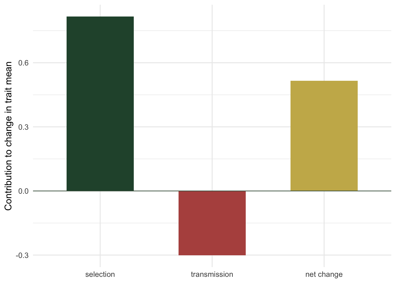
The split is informative on its own. Here the selection term is 0.816 and the transmission term is -0.300.
cat(sprintf("selection term = %+.4f\n", selection))
selection term = +0.8158
cat(sprintf("transmission term = %+.4f\n", transmission))
Selection is pushing the trait up hard, but downward transmission is bleeding off more than a third of that gain. A trait can be under strong positive selection and still barely move, or move backwards, if transmission opposes it. This is why measuring selection alone (a covariance with fitness) does not tell you how a population will evolve; you also need to know how faithfully the trait is passed on. It is the same lesson the breeder’s equation teaches with heritability, here in its most general form.
Figure 1: The observed change in the trait mean is the sum of a selection term (fitness covaries with the trait) and a transmission term (offspring drift below parents). Downward transmission cancels part of the selective gain.
Why it matters
The Price equation earns its keep when a term is itself hiding structure. If an individual’s fitness depends on a relative’s trait, the selection covariance splits into a direct and an indirect part, and, when transmission is unbiased, the condition for the trait mean to rise becomes Hamilton’s rule (Queller 1992). The same identity that separates selection from transmission separates direct selection on an individual from the selection it experiences through its kin. It also underlies the selection effect in biodiversity experiments, which is a Price covariance between the change in relative yield and monoculture yield. The equation is a lens that reappears wherever change needs to be partitioned.
An honest limit
Being an identity is a strength and a limitation. The Price equation is always true, so it never tells you whether your fitness measure is the right one, whether the covariance is causal, or whether the transmission term is mechanism or noise. It reorganises what you measured; it does not validate it. A covariance between fitness and a trait is consistent with the trait causing fitness, with an unmeasured trait causing both, or with reverse causation, exactly as any regression is. Use the Price equation to see the structure of change clearly, then bring biology to decide what the terms mean.
R version 4.5.3 (2026-03-11), aarch64-apple-darwin20
Packages: ggplot2 4.0.3
Newsletter
Get updates by email
An occasional email when tutorials are added or substantially corrected. No spam; unsubscribe anytime.
By subscribing you agree to receive these emails and confirm your address once. See the privacy policy.
ESC
Type to search the tutorials
Source Code
---title: "The Price equation in R"description: "Decompose evolutionary change in R with the Price equation: selection as a covariance plus a transmission term, an exact identity that underlies kin selection."date: "2026-07-07 09:00"categories: [evolutionary ecology, social evolution, quantitative genetics, R, ecology tutorial]image: thumbnail.pngimage-alt: "The total change in a trait mean split into a selection term and a transmission term"date-modified: "2026-10-15"---*Corrected 15 October 2026: the post said that splitting the selection covariance turns the whole Price equation into Hamilton's rule; it now says that this gives Hamilton's rule as the condition for the trait mean to rise when transmission is unbiased.**Corrected 7 October 2026: the post described the selection effect of biodiversity experiments as a covariance between yield and monoculture performance; it rests on the covariance between the change in relative yield and monoculture yield, and the text now says so.**Corrected 27 September 2026: the post said that Hamilton's rule comes from the transmission term becoming a second covariance; it now says, as in Queller (1992), that it comes from splitting the selection covariance into a direct and an indirect part.*Most of evolutionary biology is bookkeeping: how much did a trait mean move in one generation, and why. The Price equation (Price 1970) is the exact accounting identity for that move. It splits the change into a part due to selection, written as a covariance between fitness and the trait, and a part due to imperfect transmission from parent to offspring. It is not a model with assumptions to check; it is an algebraic identity, true for any population, and it is the foundation the [kin selection](../hamiltons-rule-and-kin-selection/) results are built on. This post derives it numerically in base R.## The identityFor a population of parents with trait value `z` and fitness `w` (number of offspring), and a transmission change `delta` for each parent's offspring, the change in the mean trait is$$\bar{w}\,\Delta\bar{z} = \operatorname{Cov}(w, z) + \operatorname{E}(w\,\delta).$$The first term is selection: if fitness covaries with the trait, the mean shifts. The second is transmission: if offspring differ systematically from parents (mutation, biased inheritance, developmental drift), that shifts the mean too. Here is a population where the trait raises fitness but offspring drift downward from their parents.```{r}#| label: priceset.seed(439)n <-2000z <-rnorm(n, 10, 2)w <-pmax(0, 1+0.25* (z -10) +rnorm(n, 0, 0.5)) # fitness rises with zdelta <-rnorm(n, -0.3, 0.4) # offspring drift below parentszbar <-mean(z); wbar <-mean(w)dz_obs <-sum(w * (z + delta)) /sum(w) - zbar # actual change in the meanselection <-mean((w - wbar) * (z - zbar)) / wbar # Cov(w, z) / wbartransmission <-mean(w * delta) / wbar # E(w delta) / wbarcat(sprintf("observed change = %.5f\n", dz_obs))cat(sprintf("selection + transmission = %.5f\n", selection + transmission))cat(sprintf("difference = %.1e\n", dz_obs - (selection + transmission)))```The two sides agree: the difference printed above is zero up to floating-point rounding. That exactness is the point. The Price equation does not approximate the change; it partitions it. Any evolutionary change, in any population, splits cleanly into these two pieces.## Reading the two termsThe split is informative on its own. Here the selection term is `0.816` and the transmission term is `-0.300`.```{r}#| label: termscat(sprintf("selection term = %+.4f\n", selection))cat(sprintf("transmission term = %+.4f\n", transmission))cat(sprintf("net change = %+.4f\n", selection + transmission))```Selection is pushing the trait up hard, but downward transmission is bleeding off more than a third of that gain. A trait can be under strong positive selection and still barely move, or move backwards, if transmission opposes it. This is why measuring selection alone (a covariance with fitness) does not tell you how a population will evolve; you also need to know how faithfully the trait is passed on. It is the same lesson the [breeder's equation](../the-breeders-equation/) teaches with heritability, here in its most general form.```{r}#| label: fig-decomp#| fig-cap: "The observed change in the trait mean is the sum of a selection term (fitness covaries with the trait) and a transmission term (offspring drift below parents). Downward transmission cancels part of the selective gain."#| fig-alt: "A bar chart showing a large positive selection bar, a negative transmission bar, and their smaller positive sum."library(ggplot2)te_canvas <-theme(plot.background =element_rect(fill ="#f5f4ee", colour =NA),panel.background =element_rect(fill ="#f5f4ee", colour =NA))d <-data.frame(part =factor(c("selection", "transmission", "net change"),levels =c("selection", "transmission", "net change")),val =c(selection, transmission, selection + transmission))ggplot(d, aes(part, val, fill = part)) +geom_col(width =0.6) +geom_hline(yintercept =0, colour ="#46604a", linewidth =0.4) +scale_fill_manual(values =c(selection ="#275139", transmission ="#b5534e", "net change"="#c9b458"),guide ="none") +labs(x =NULL, y ="Contribution to change in trait mean") +theme_minimal(base_size =12) + te_canvas```## Why it mattersThe Price equation earns its keep when a term is itself hiding structure. If an individual's fitness depends on a *relative's* trait, the selection covariance splits into a direct and an indirect part, and, when transmission is unbiased, the condition for the trait mean to rise becomes Hamilton's rule (Queller 1992). The same identity that separates selection from transmission separates direct selection on an individual from the selection it experiences through its kin. It also underlies the [selection effect in biodiversity experiments](../complementarity-and-selection-effects/), which is a Price covariance between the change in relative yield and monoculture yield. The equation is a lens that reappears wherever change needs to be partitioned.## An honest limitBeing an identity is a strength and a limitation. The Price equation is always true, so it never tells you whether your fitness measure is the right one, whether the covariance is causal, or whether the transmission term is mechanism or noise. It reorganises what you measured; it does not validate it. A covariance between fitness and a trait is consistent with the trait causing fitness, with an unmeasured trait causing both, or with reverse causation, exactly as any [regression is](../confounding-and-backdoor-adjustment/). Use the Price equation to see the structure of change clearly, then bring biology to decide what the terms mean.## ReferencesPrice GR 1970. Nature 227(5257):520-521 (10.1038/227520a0)Price GR 1972. Annals of Human Genetics 35(4):485-490 (10.1111/j.1469-1809.1957.tb01874.x)Queller DC 1992. Evolution 46(2):376-380 (10.1111/j.1558-5646.1992.tb02045.x)Frank SA 1998. Foundations of Social Evolution. Princeton University Press. ISBN 978-0691059341## Related tutorials- [Hamilton's rule and kin selection](../hamiltons-rule-and-kin-selection/)- [Relatedness as a regression](../relatedness-as-a-regression/)- [Multilevel selection and group structure](../multilevel-selection-and-groups/)- [Complementarity and selection effects](../complementarity-and-selection-effects/)