---
title: "Complementarity and selection effects"
description: "Why the biodiversity selection effect is a covariance, not a mechanism: the Price-equation link, and what the additive partition cannot tell you about cause."
date: "2026-06-29 11:00"
categories: [ecology tutorial, R, biodiversity, ecosystem function, community ecology]
image: thumbnail.png
date-modified: "2026-10-15"
image-alt: "Per-species relative-yield deviations plotted against monoculture yield: six dark points sit along an upward sloping orange line that crosses a dashed horizontal reference line."
---
*Corrected 15 October 2026: the post said that in the second mixture the gains are concentrated in a few species; most of the species gain more than under the uniform boost, so the text now says the gains are uneven, with some species gaining strongly and one barely benefiting.*
*Corrected 7 October 2026: the post credited the Price-equation reading of the selection effect to Fox's paper on species loss and said the word "selection" was borrowed from statistics; it now credits the analogy to Loreau and Hector, and cites Fox's Ecology Letters paper for showing that the analogy with natural selection is only partial.*
*Corrected 27 September 2026: the caption of the instability figure said the monoculture yield shrinks from right to left; the axis is reversed, so it now says left to right, as drawn.*
```{r setup}
#| code-fold: true
#| code-summary: "Setup: packages, colours and plot theme"
#| results: hide
#| message: false
#| warning: false
knitr::opts_chunk$set(echo = TRUE, message = FALSE, warning = FALSE,
                      dev = "png", dpi = 120, fig.path = "figures/",
                      fig.width = 7, fig.height = 4.4)
library(ggplot2)
theme_te <- theme_minimal(base_size = 12) +
  theme(panel.background = element_rect(fill = "#f5f4ee", colour = NA),
        plot.background  = element_rect(fill = "#f5f4ee", colour = NA),
        panel.grid.minor = element_blank(),
        plot.title = element_text(face = "bold", size = 12),
        strip.text = element_text(face = "bold"))
theme_set(theme_te)
col_a <- "#3a6b52"; col_b <- "#b5651d"; col_ref <- "#555555"

lh <- function(M, RYo, RYe) {
  dRY <- RYo - RYe; N <- length(M)
  c(dY = sum(dRY * M), comp = N * mean(dRY) * mean(M),
    sel = N * mean((dRY - mean(dRY)) * (M - mean(M))))
}

## two mechanisms, identical partition
set.seed(389)
M   <- round(runif(6, 80, 700)); RYe <- rep(1/6, 6); m <- 0.08
dRY_A <- rep(m, 6)
raw   <- c(-0.05, 0.22, 0.05, 0.14, -0.02, 0.10)
bcoef <- sum((raw - mean(raw)) * (M - mean(M))) / sum((M - mean(M))^2)
dRY_B <- m + (raw - mean(raw)) - bcoef * (M - mean(M))
pA <- lh(M, RYe + dRY_A, RYe); pB <- lh(M, RYe + dRY_B, RYe)
covB <- mean((dRY_B - mean(dRY_B)) * (M - mean(M)))

## monoculture-reference instability
Mbase <- rep(300, 6); Yobs <- c(120,110,130,125,115,140); RYe6 <- rep(1/6, 6)
frac  <- seq(1, 0.05, by = -0.05)
inst  <- data.frame()
for (f in frac) {
  M6 <- Mbase; M6[1] <- 300 * f
  p  <- lh(M6, Yobs / M6, RYe6)
  inst <- rbind(inst, data.frame(frac = f, comp = p["comp"], sel = p["sel"], net = p["dY"]))
}
net_full <- inst$net[inst$frac == 1]; comp_full <- inst$comp[inst$frac == 1]
i_lo <- which.min(inst$frac)
RYo1_lo <- Yobs[1] / (300 * min(frac))
```
The [additive partition](../partitioning-the-net-biodiversity-effect/) hands you two numbers, a complementarity effect and a selection effect, and it is tempting to read them as two mechanisms: complementarity means the species help each other, selection means one species wins. That reading is too generous. This post is about what the two numbers actually are, and where reading them as mechanisms goes wrong.
## Selection is a covariance
The selection effect is *N* times the covariance between monoculture yield and the change in relative yield. Written that way, it is exactly the shape of the selection term in the Price equation, where evolutionary change is split into a covariance between fitness and a trait plus a transmission term. Loreau and Hector 2001 Nature 412(6842):72-76 presented their partition as analogous to the Price equation: on that reading, the biodiversity selection effect is a statistical selection differential, with monoculture yield playing the role of the trait and the change in relative yield playing the role of fitness.
That analogy is the warning. A covariance is a description of who over- and under-performs; it is silent on why. A positive selection effect says the productive species happen to overperform in this mixture. It does not say they outcompete anyone, and it certainly does not name a biological process. The word "selection" echoes natural selection, but Fox 2005 Ecology Letters 8(8):846-856 used the Price equation to show that the covariance only partly reflects dominance by species with particular traits at the expense of other species, so the analogy with natural selection is only partial.
## The same numbers, two different ecologies
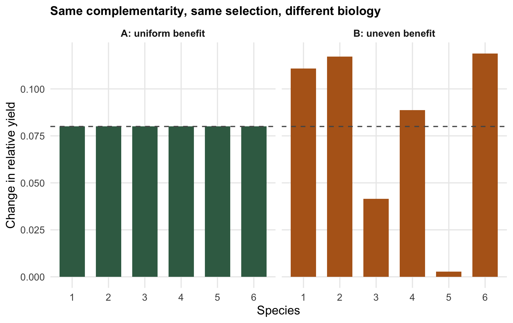
Here is the sharp version. Take six species and build two mixtures that a field ecologist would describe completely differently. In the first, every species does a little better than expected: a uniform boost, the picture you would draw for resource partitioning. In the second, the benefits are lopsided, with some species gaining strongly and one barely benefiting, the picture you would draw for facilitation by a nurse species, and the gains are arranged so they do not track monoculture yield.
```{r two-mechanisms}
m     <- 0.08
dRY_A <- rep(m, 6)                                   # uniform: "resource partitioning"
raw   <- c(-0.05, 0.22, 0.05, 0.14, -0.02, 0.10)     # uneven: "facilitation"
bcoef <- sum((raw - mean(raw)) * (M - mean(M))) / sum((M - mean(M))^2)
dRY_B <- m + (raw - mean(raw)) - bcoef * (M - mean(M))
rbind(A = round(lh(M, RYe + dRY_A, RYe), 4),
      B = round(lh(M, RYe + dRY_B, RYe), 4))
```
Both mixtures return a net effect of `r sprintf("%.1f", pA["dY"])` g/m^2^, a complementarity effect of `r sprintf("%.1f", pA["comp"])`, and a selection effect of `r sprintf("%.1f", pA["sel"])`. The partition is identical to the last decimal, because the covariance of the second pattern with monoculture yield was set to zero, and in the run it is zero up to floating-point rounding. Yet the per-species story is not the same at all: in mixture A everyone gains equally, in mixture B the gains are uneven, with some species gaining strongly and one barely benefiting.
```{r fp-guard-1}
#| include: false
stopifnot(abs(covB) < 1e-10 * sd(M) * sd(dRY_B))
```
```{r fig-mechanisms}
#| fig-cap: "Two per-species patterns of relative-yield change. They look different, but both have the same mean and no covariance with monoculture yield, so the partition returns identical complementarity and zero selection for each."
#| fig-alt: "Two bar panels of relative-yield change across six species; the left panel is flat and equal, the right panel is uneven with one near-zero bar, yet both give the same complementarity and selection values."
dm <- rbind(
  data.frame(mech = "A: uniform benefit", sp = 1:6, dRY = dRY_A),
  data.frame(mech = "B: uneven benefit",  sp = 1:6, dRY = dRY_B))
ggplot(dm, aes(factor(sp), dRY, fill = mech)) +
  geom_col(width = 0.7) +
  geom_hline(yintercept = m, colour = col_ref, linetype = "dashed") +
  facet_wrap(~mech) +
  scale_fill_manual(values = c("A: uniform benefit" = col_a, "B: uneven benefit" = col_b), guide = "none") +
  labs(x = "Species", y = "Change in relative yield",
       title = "Same complementarity, same selection, different biology")
```
The partition sees only the mean of the deviations and their covariance with monoculture yield. Any two mixtures that share those two summaries are indistinguishable to it, however different the underlying interactions. So a large complementarity effect corroborates that something beyond a simple average is going on; it cannot tell you whether that something is resource partitioning, facilitation, or release from a shared enemy. Naming the mechanism needs the mechanism measured directly: rooting depth, nitrogen fixation, herbivore loads, not the partition alone.
## The monoculture references are load-bearing
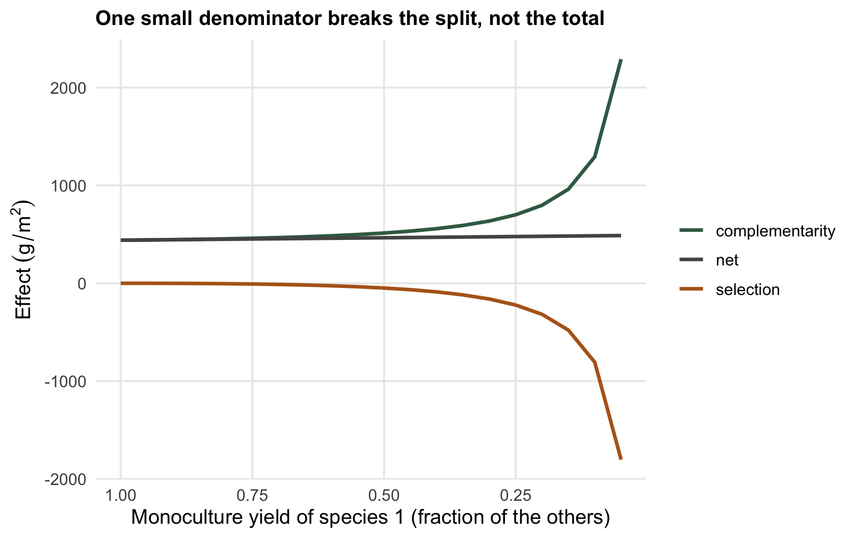
Every relative yield is a species' mixture yield divided by its monoculture yield, so the whole partition rests on the monocultures. When a species performs well in monoculture the division is stable. When a species nearly fails in monoculture, its relative yield explodes, and the split follows.
```{r instability}
Mbase <- rep(300, 6); Yobs <- c(120,110,130,125,115,140)
shrink <- function(f) { M6 <- Mbase; M6[1] <- 300 * f; lh(M6, Yobs / M6, rep(1/6,6)) }
rbind(full = round(shrink(1.00), 1), nearly_zero = round(shrink(0.05), 1))
```
At full strength the partition is stable. Shrink one species' monoculture yield to a twentieth of the others and its relative yield climbs to `r sprintf("%.0f", RYo1_lo)`; the complementarity effect swings from `r sprintf("%.0f", comp_full)` to `r sprintf("%.0f", inst$comp[i_lo])` g/m^2^ and selection swings by as much in the other direction, while the net effect barely moves. The partition has become an artefact of one small denominator.
```{r fig-instability}
#| fig-cap: "As one species' monoculture yield shrinks toward zero (left to right), the complementarity and selection effects diverge while the net effect stays almost flat. The split is unstable, the total is not."
#| fig-alt: "Line plot: as a monoculture reference shrinks toward zero, complementarity rises steeply and selection falls steeply while the net effect stays roughly constant."
il <- rbind(data.frame(frac = inst$frac, effect = "complementarity", val = inst$comp),
            data.frame(frac = inst$frac, effect = "selection",       val = inst$sel),
            data.frame(frac = inst$frac, effect = "net",             val = inst$net))
ggplot(il, aes(frac, val, colour = effect)) +
  geom_line(linewidth = 1) +
  scale_x_reverse() +
  scale_colour_manual(values = c(complementarity = col_a, selection = col_b, net = col_ref)) +
  labs(x = "Monoculture yield of species 1 (fraction of the others)",
       y = expression(Effect~(g/m^2)), colour = NULL,
       title = "One small denominator breaks the split, not the total")
```
This is why the design of the monocultures matters as much as the mixtures: they must be grown at the same density and in the same conditions, and species that cannot persist in monoculture sit awkwardly in the method. The checking post makes this a formal diagnostic.
## Using the partition well
None of this makes the partition useless. It is exact, it is cheap, and it separates two genuinely different aggregate patterns that a single net number hides. The discipline is in the reading. Report both effects, treat "selection" as the covariance it is, and remember that its interpretation is still argued over in the literature (Pillai and Gouhier 2019 Ecology 100(7):e02645 go as far as calling the standard measures spurious in some settings, which drew replies). Corroborate a complementarity signal with a measured process before you call it niche partitioning. The partition is a lens on the pattern, not a verdict on the cause.
## References
- Fox JW 2005. Ecology Letters 8(8):846-856 (10.1111/j.1461-0248.2005.00795.x).
- Fox JW 2006. Ecology 87(11):2687-2696 (10.1890/0012-9658(2006)87[2687:UTPETP]2.0.CO;2).
- Loreau M, Hector A 2001. Nature 412(6842):72-76 (10.1038/35083573).
- Pillai P, Gouhier TC 2019. Ecology 100(7):e02645 (10.1002/ecy.2645).
## Related tutorials
- [Partitioning the net biodiversity effect](../partitioning-the-net-biodiversity-effect/)
- [Checking a biodiversity-function analysis](../checking-a-biodiversity-ecosystem-function-analysis/)
- [Biodiversity and ecosystem function in R](../biodiversity-and-ecosystem-function/)
- [The Price equation](../the-price-equation/)